Project-1: Modelling an electric Car with Li-ion battery
AIM:- TO CREATE A MATLAB MODEL OF AN ELECTRIC CAR WITH LITHIUM ION BATTERIES
BLOCKS USED:-
Drive Cycle Source
Description
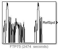
The Drive Cycle Source block generates a standard or user-specified longitudinal drive cycle. The block output is the specified vehicle longitudinal speed, which you can use to:
-
Predict the engine torque and fuel consumption that a vehicle requires to achieve desired speed and acceleration for a given gear shift reference.
-
Produce realistic velocity and shift references for closed loop acceleration and braking commands for vehicle control and plant models.
-
Study, tune, and optimize vehicle control, system performance, and system robustness over multiple drive cycles.
-
Identify the faults within tolerances specified by standardized tests, including:
-
EPA dynamometer driving schedules1
-
Worldwide Harmonised Light Vehicle Test Procedure (WLTP) laboratory tests2
-
For the drive cycles, you can use:
-
Drive cycles from predefined sources. By default, the block includes the
FTP–75drive cycle. To install additional drive cycles from a support package, see Install Drive Cycle Data. The support package has drive cycles that include the gear shift schedules, for exampleJC08andCUEDC. -
Workspace variables that define your own drive cycles.
-
.
mat, .xls, .xlsx, or .txtfiles. -
Wide open throttle (WOT) parameters, including initial and nominal reference speed, deceleration start time, and final reference speed.
Create Subsystems
As a model increases in size and complexity, you can simplify it by grouping blocks into subsystems. A subsystem is a set of blocks that you group into a single Subsystem block.
Using subsystems:
-
Establishes a hierarchical block diagram where a Subsystem block is on one layer and the blocks that make up the subsystem are on another.
-
Keeps functionally related blocks together.
-
Helps reduce the number of blocks displayed in your model window.
-
Establishes an interface with inputs and outputs.
When you make a copy of a subsystem, that copy is independent of the source subsystem. To reuse the contents of a subsystem across a model or across models, consider referenced subsystems, referenced models, or subsystems linked to a block in a custom library. For more information, see Choose Among Types of Model Components.
Add, Subtract, Sum of Elements, Sum

Description
The Sum block performs addition or subtraction on its inputs. The Add, Subtract, Sum of Elements, and Sum blocks are identical blocks. This block can add or subtract scalar, vector, or matrix inputs. It can also collapse the elements of a signal and perform a summation.
You specify the operations of the block with the List of signs parameter with plus (+), minus (-), and spacer (|).
-
The number of
+and-characters equals the number of inputs. For example,+-+requires three inputs. The block subtracts the second (middle) input from the first (top) input, and then adds the third (bottom) input. -
A spacer character creates extra space between ports on the block icon.
-
If performing only addition, you can use a numerical value equal to the number of inputs.
-
If only there is only one input port, a single
+or-adds or subtracts the elements over all dimensions or in the specified dimension.
The Sum block first converts the input data type to its accumulator data type, then performs the specified operations. The block converts the result to its output data type using the specified rounding and overflow modes.
Discrete PID Controller
Description
The Discrete PID Controller block implements a PID controller (PID, PI, PD, P only, or I only). The block is identical to the PID Controller block with the Time domain parameter set to Discrete-time.
The block output is a weighted sum of the input signal, the integral of the input signal, and the derivative of the input signal. The weights are the proportional, integral, and derivative gain parameters. A first-order pole filters the derivative action.
The block supports several controller types and structures. Configurable options in the block include:
-
Controller type (PID, PI, PD, P only, or I only) — See the Controller parameter.
-
Controller form (Parallel or Ideal) — See the Form parameter.
-
Time domain (continuous or discrete) — See the Time domain parameter.
-
Initial conditions and reset trigger — See the Source and External reset parameters.
-
Output saturation limits and built-in anti-windup mechanism — See the Limit output parameter.
-
Signal tracking for bumpless control transfer and multiloop control — See the Enable tracking mode parameter.
As you change these options, the internal structure of the block changes by activating different variant subsystems. (For more information, see Variant Subsystems). To examine the internal structure of the block and its variant subsystems, right-click the block and select Mask > Look Under Mask.
Control Configuration
In one common implementation, the PID Controller block operates in the feedforward path of a feedback loop.
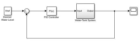
The input of the block is typically an error signal, which is the difference between a reference signal and the system output. For a two-input block that permits setpoint weighting, see Discrete PID Controller (2DOF).
PID Gain Tuning
The PID controller gains are tunable either manually or automatically. Automatic tuning requires Simulink® Control Design™ software. For more information about automatic tuning, see the Select tuning method parameter.
Saturation

Description
The Saturation block produces an output signal that is the value of the input signal bounded to the upper and lower saturation values. The upper and lower limits are specified by the parameters Upper limit and Lower limit.
Transfer Fcn

Description
The Transfer Fcn block models a linear system by a transfer function of the Laplace-domain variable s. The block can model single-input single-output (SISO) and single-input multiple-output (SIMO) systems.
Conditions for Using This Block
The Transfer Fcn block assumes the following conditions:
-
The transfer function has the form
H(s)=y(s)u(s)=num(s)den(s)=num(1)snn−1+num(2)snn−2+…+num(nn)den(1)snd−1+den(2)snd−2+…+den(nd),
where u and y are the system input and outputs, respectively, nn and nd are the number of numerator and denominator coefficients, respectively. num(s) and den(s) contain the coefficients of the numerator and denominator in descending powers of s.
-
The order of the denominator must be greater than or equal to the order of the numerator.
-
For a multiple-output system, all transfer functions have the same denominator and all numerators have the same order.
Modeling a Single-Output System
For a single-output system, the input and output of the block are scalar time-domain signals. To model this system:
-
Enter a vector for the numerator coefficients of the transfer function in the Numerator coefficients field.
-
Enter a vector for the denominator coefficients of the transfer function in the Denominator coefficients field.
Modeling a Multiple-Output System
For a multiple-output system, the block input is a scalar and the output is a vector, where each element is an output of the system. To model this system:
-
Enter a matrix in the Numerator coefficients field.
Each row of this matrix contains the numerator coefficients of a transfer function that determines one of the block outputs.
-
Enter a vector of the denominator coefficients common to all transfer functions of the system in the Denominator coefficients field.
Specifying Initial Conditions
A transfer function describes the relationship between input and output in Laplace (frequency) domain. Specifically, it is defined as the Laplace transform of the response (output) of a system with zero initial conditions to an impulse input.
Operations like multiplication and division of transfer functions rely on zero initial state. For example, you can decompose a single complicated transfer function into a series of simpler transfer functions. Apply them sequentially to get a response equivalent to that of the original transfer function. This will not be correct if one of the transfer functions assumes a non-zero initial state. Furthermore, a transfer function has infinitely many time domain realizations, most of whose states do not have any physical meaning.
For these reasons, Simulink® presets the initial conditions of the Transfer Fcn block to zero. To specify initial conditions for a given transfer function, convert the transfer function to its controllable, canonical state-space realization using tf2ss . Then, use the State-Space block. The tf2ss utility provides the A, B, C, and D matrices for the system.
For more information, type help tf2ss or see the Control System Toolbox™ documentation.
Transfer Function Display on the Block
The Transfer Fcn block displays the transfer function depending on how you specify the numerator and denominator parameters.
-
If you specify each parameter as an expression or a vector, the block shows the transfer function with the specified coefficients and powers of s. If you specify a variable in parentheses, the block evaluates the variable.
For example, if you specify Numerator coefficients as
[3,2,1]and Denominator coefficients as(den), wheredenis[7,5,3,1], the block looks like this: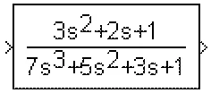
-
If you specify each parameter as a variable, the block shows the variable name followed by
(s).For example, if you specify Numerator coefficients as
numand Denominator coefficients asden, the block looks like this: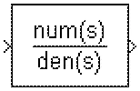
Delay

Description
The Delay block outputs the input of the block after a delay. The block determines the delay time based on the value of the Delay length parameter. The block supports:
-
Variable delay length
-
Specification of the initial condition from an input port
-
State storage
-
Using a circular buffer instead of an array buffer for state storage
-
Resetting the state to the initial condition with an external reset signal
-
Controlling execution of the block at every time step with an external enable signal
The initial block output depends on several factors such as the Initial condition parameter and the simulation start time. For more information, see Initial Block Output. The External reset parameter determines if the block output resets to the initial condition on triggering. The Show enable port parameter determines if the block execution is controlled in every time step by an external enable signal.
Initial Block Output
The output in the first few time steps of the simulation depends on the block sample time, the delay length, and the simulation start time. The block supports specifying or inheriting discrete sample times to determine the time interval between samples. For more information, see Specify Sample Time.
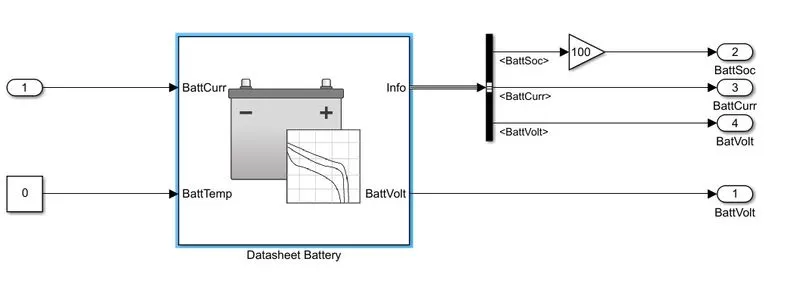
Datasheet Battery
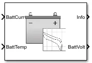
Description
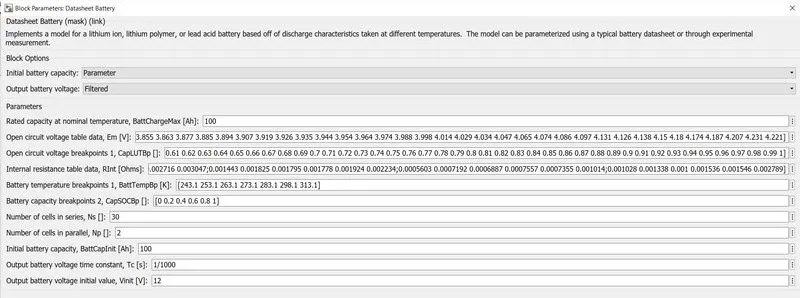
The Datasheet Battery block implements a lithium-ion, lithium-polymer, or lead-acid battery that you can parameterize using manufacturer data. To create the open-circuit voltage and internal resistance parameters that you need for the block, use the manufacturer discharge characteristics by temperature data. For an example, see Generate Parameter Data for Datasheet Battery Block.
To determine the battery output voltage, the block uses lookup tables for the battery open-circuit voltage and the internal resistance. The lookup tables are functions of the state-of charge (SOC) and battery temperature, characterizing the battery performance at various operating points:
Em=f(SOC)Rint=f(T,SOC)
Bus Selector

Description
The Bus Selector block outputs the elements you select from the input bus. The block can output the selected elements separately or in a new virtual bus.
Gain

Description
The Gain block multiplies the input by a constant value (gain). The input and the gain can each be a scalar, vector, or matrix.
You specify the value of gain in the Gain parameter. The Multiplication parameter lets you specify element-wise or matrix multiplication. For matrix multiplication, this parameter also lets you indicate the order of the multiplicands.
Gain is converted from doubles to the data type specified in the block mask offline using round-to-nearest and saturation. The input and gain are then multiplied, and the result is converted to the output data type using the specified rounding and overflow modes.
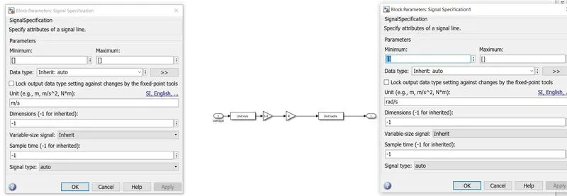
Signal Specification
Description
The Signal Specification block allows you to specify the attributes of the signal connected to its input and output ports. If the specified attributes conflict with the attributes specified by the blocks connected to its ports, Simulink® software displays an error when it compiles the model. For example, at the beginning of a simulation, if no conflict exists, Simulink eliminates the Signal Specification block from the compiled model. In other words, the Signal Specification block is a virtual block. It exists only to specify the attributes of a signal and plays no role in the simulation of the model.
You can use the Signal Specification block to ensure that the actual attributes of a signal meet desired attributes. For example, suppose that you and a colleague are working on different parts of the same model. You use Signal Specification blocks to connect your part of the model with your colleague's. If your colleague changes the attributes of a signal without informing you, the attributes entering the corresponding Signal Specification block do not match. When you try to simulate the model, you get an error.
You can also use the Signal Specification block to ensure correct propagation of signal attributes throughout a model. However, if some blocks have unspecified attributes for the signals they accept or output, the model does not have enough information to propagate attributes correctly. In these cases, the Signal Specification block can provide the information Simulink needs. Using the Signal Specification block also helps speed up model compilation when blocks are missing signal attributes.
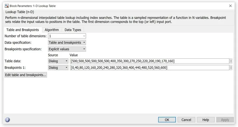
n-D Lookup Table

Description
Supported Block Operations
The 1-D, 2-D, and n-D Lookup Table blocks evaluate a sampled representation of a function in N variables
y=F(x1,x2,x3,...,xN)
where the function F can be empirical. The block maps inputs to an output value by looking up or interpolating a table of values you define with block parameters. The block supports flat (constant), linear (linear point-slope), Lagrange (linear Lagrange), nearest, cubic-spline, and Akima spline interpolation methods. You can apply these methods to a table of any dimension from 1 through 30.
In the following block, the first input identifies the first dimension (row) breakpoints, the second input identifies the second dimension (column) breakpoints, and so on.
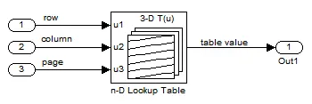
See Port Location After Rotating or Flipping for a description of the port order for various block orientations.
When the Math and Data Types > Use algorithms optimized for row-major array layout configuration parameter is set, the 2-D and n-D Lookup Table block behavior changes from column-major to row-major. For these blocks, the column-major and row-major algorithms may differ in the order of the output calculations, possibly resulting in slightly different numerical values. This capability requires a Simulink® Coder™ or Embedded Coder® license. For more information on row-major support, see Code Generation of Matrices and Arrays (Simulink Coder).
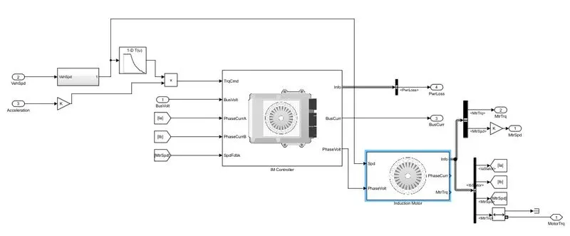
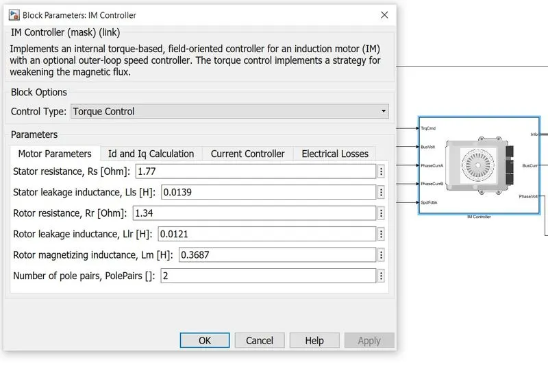
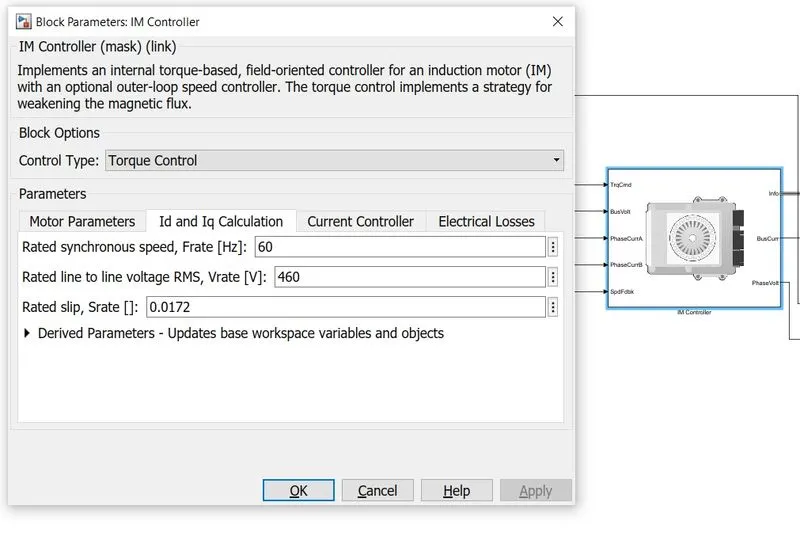
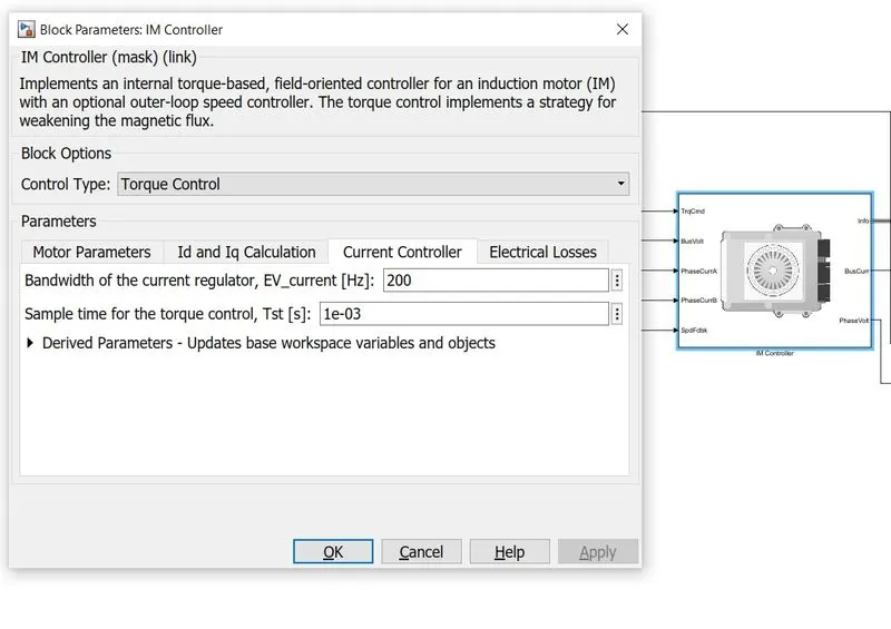
IM Controller
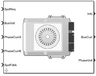
Description
The IM Controller block implements an internal torque-based, field-oriented controller for an induction motor (IM) with an optional outer-loop speed controller. The torque control implements a strategy to control the motor flux. You can specify either speed or torque control.
The IM Controller implements equations for speed control, torque determination, regulators, transforms, and motors.
The figure illustrates the information flow in the block.
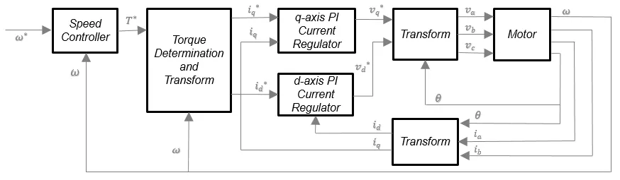
The block implements equations that use these variables.
| ω |
Rotor speed |
| ω* |
Rotor speed command |
| T* |
Torque command |
|
id i*d |
d-axis current d-axis current command |
|
iq i*q |
q-axis current q-axis current command |
|
vd, v*d |
d-axis voltage d-axis voltage command |
|
vq v*q |
q-axis voltage q-axis voltage command |
| va, vb, vc |
Stator phase a, b, c voltages |
| ia, ib, ic |
Stator phase a, b, c currents |
Speed Controller
To implement the speed controller, select the Control Type parameter Speed Control. If you select the Control Type parameter Torque Control, the block does not implement the speed controller.
The speed controller determines the torque command by implementing a state filter, and calculating the feedforward and feedback commands. If you do not implement the speed controller, input a torque command to the IM Controller block.
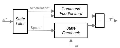
The state filter is a low-pass filter that generates the acceleration command based on the speed command. On the Speed Controller tab:
-
To make the speed-command lag time negligible, specify a Bandwidth of the state filter parameter.
-
To calculate a Speed regulation time constant, Ksf gain based on the state filter bandwidth, select Calculate Speed Regulator Gains.
The discrete form of characteristic equation is given by:
z+KsfTsm−1
The filter calculates the gain using this equation.
Ksf=1−exp(−Tsm2πEVsf)Tsm
The equation uses these variables.
| EVsf |
Bandwidth of the speed command filter |
| Tsm |
Motion controller sample time |
| Ksf |
Speed regulator time constant |
To generate the state feedback torque, the block uses the filtered speed error signal from the state filter. The feedback torque calculation also requires gains for speed regulator.
On the Speed Controller tab, select Calculate Speed Regulator Gains to compute:
-
Proportional gain, ba
-
Angular gain, Ksa
-
Rotational gain, Kisa
Induction Motor
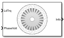
Description
The Induction Motor block implements a three-phase induction motor. The block uses the three-phase input voltages to regulate the individual phase currents, allowing control of the motor torque or speed.
By default, the block sets the Simulation Type parameter to Continuous to use a continuous sample time during simulation. If you want to generate code for fixed-step double- and single-precision targets, considering setting the parameter to Discrete. Then specify a Sample Time, Ts parameter.
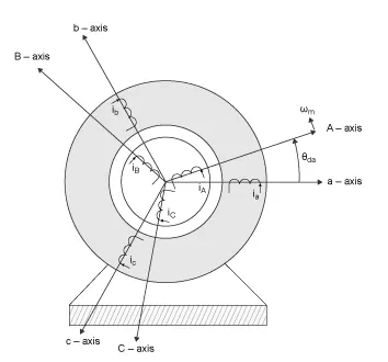
Three-Phase Sinusoidal Model Electrical System
The block implements equations that are expressed in a stationary rotor reference (qd) frame. The d-axis aligns with the a-axis. All quantities in the rotor reference frame are referred to the stator.
Goto

Description
The Goto block passes its input to its corresponding From blocks. The input can be a real- or complex-valued signal or vector of any data type. From and Goto blocks allow you to pass a signal from one block to another without actually connecting them.
A Goto block can pass its input signal to more than one From block, although a From block can receive a signal from only one Goto block. The input to that Goto block is passed to the From blocks associated with it as though the blocks were physically connected.
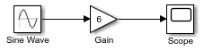
For example, this model uses a Goto block and a From block.

An equivalent model passes the Sine Wave block signal directly to the Gain block.
Goto blocks and From blocks are matched by the use of Goto tags.
The Tag Visibility parameter determines whether the location of From blocks that access the signal is limited:
-
local(default) — From and Goto blocks that use the same tag must be in the same subsystem. A local tag name is enclosed in brackets ([]). -
scoped— From and Goto blocks that use the same tag must be either:-
In the same subsystem.
-
At any level in the model hierarchy below the Goto Tag Visibility block that does not entail crossing a nonvirtual subsystem boundary. In other words, they must be within the boundary of an atomic, conditionally executed, or function-call subsystem or a model reference.
A scoped tag name is enclosed in braces (
{}). -
-
global— From and Goto blocks using the same tag can be anywhere in the model except in locations that span nonvirtual subsystem boundaries.
The rule that From-Goto block connections cannot cross nonvirtual subsystem boundaries has the following exception. A Goto block connected to a state port in one conditionally executed subsystem is visible to a From block inside another conditionally executed subsystem.
Use local tags when the Goto and From blocks using the same tag name reside in the same subsystem. You must use global or scoped tags when the Goto and From blocks using the same tag name reside in different subsystems. When you define a tag as global, all uses of that tag access the same signal. A tag defined as scoped can be used in more than one place in the model.
Selecting a Goto block highlights the corresponding From blocks.
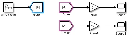
Similarly, selecting a From block highlights the corresponding Goto block.

When a subsystem contains a corresponding Goto or From block, the Subsystem block is highlighted.
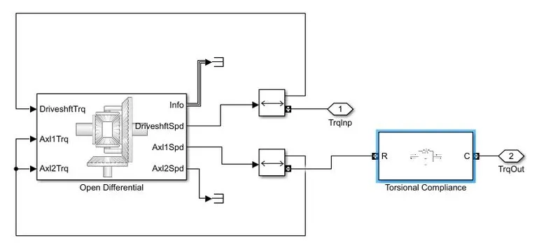
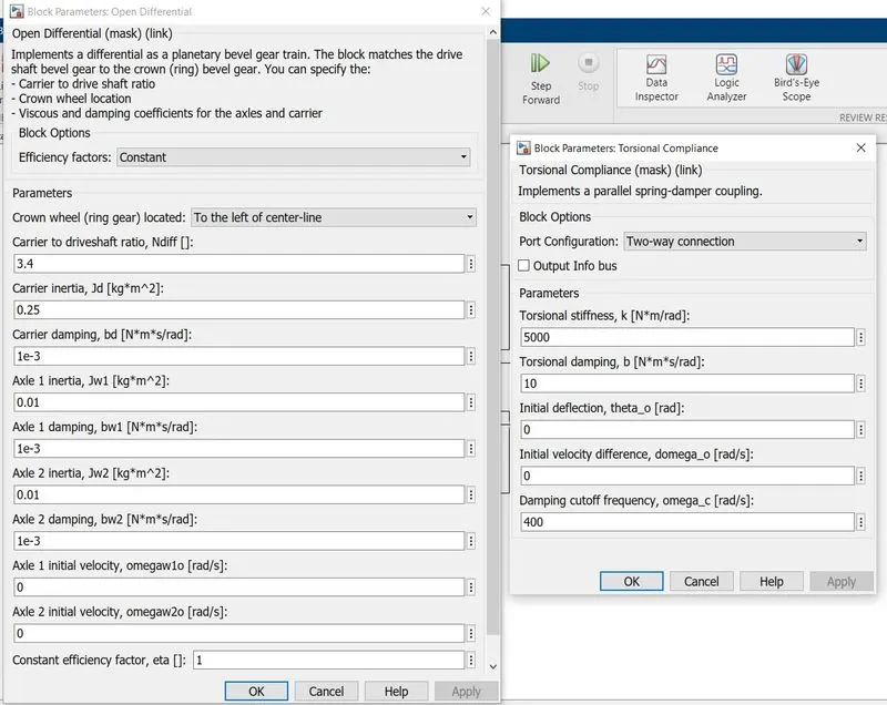
Open Differential
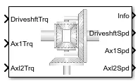
Description
The Open Differential block implements a differential as a planetary bevel gear train. The block matches the driveshaft bevel gear to the crown (ring) bevel gear. You can specify:
-
Carrier-to-driveshaft ratio
-
Crown wheel location
-
Viscous and damping coefficients for the axles and carrier
Use the Open Differential block to:
-
Dynamically couple the post-transmission driveshaft to the wheel axles or universal joints
-
Model simplified or older drivetrains when optimal traction control does not require passive or active torque vectoring
-
Model mechanical power splitting in generic gearbox and drive line scenarios
The block is suitable for use in hardware-in-the-loop (HIL) and optimization workflows. All the parameters are tunable.
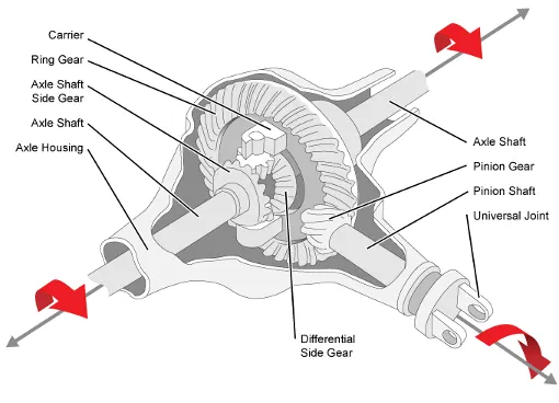
The block uses a coordinate system that produces positive tire and vehicle motion for standard engine, transmission, and differential configurations. The arrows indicate positive motion.
Terminator

Description
Use the Terminator block to cap blocks whose output ports do not connect to other blocks. If you run a simulation with blocks having unconnected output ports, Simulink® issues warning messages. Using Terminator blocks to cap those blocks helps prevent warning messages.
Two-Way Connection

Description
The Two-Way Connection block has a two-way connector port, which transports Simulink® signals both ways. You connect this port to another two-way connector port. The schematic below illustrates how the two-way connection works. It carries the signal Signal1 from the input port of the first Two-Way Connection block to the output port of the second Two-Way Connection block, and at the same time carries the signal Signal2 from the input port of the second Two-Way Connection block to the output port of the first Two-Way Connection block.
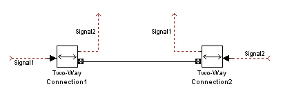
The Two-Way Connection block supports invariant model architecture for top-down or bottom-up design. It lets you build subsystems as Simulink models, based on signals, and then connect them as if they are physical systems. Place the Two-Way Connection blocks inside the subsystem and connect them to the Connection Port (Simscape) blocks. Then the ports on the subsystem boundary appear as two-way connector ports  .
.
Torsional Compliance
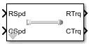
Description
The Torsional Compliance block implements a parallel spring-damper to couple two rotating driveshafts. The block uses the driveshaft angular velocities, torsional stiffness, and torsional damping to determine the torques.
TR=−(ωR−ωC)b−θk
TC=(ωR−ωC)b+θk˙
θ=(ωR−ωC)
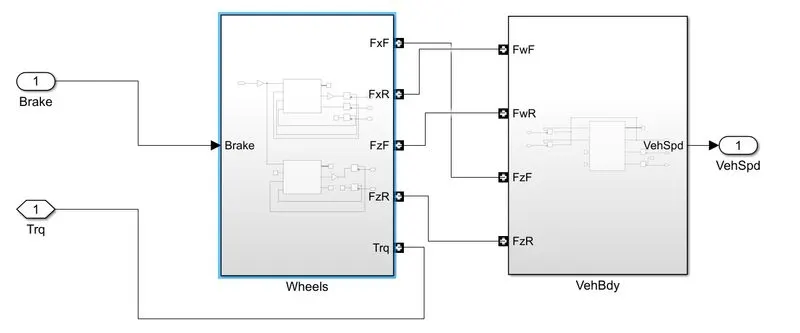
Longitudinal Wheel
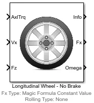
Description
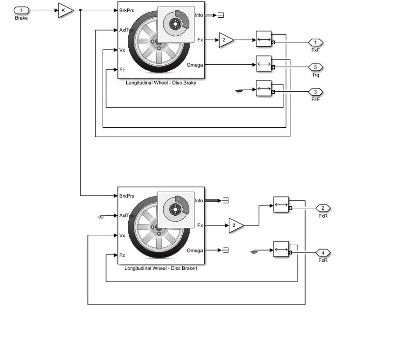
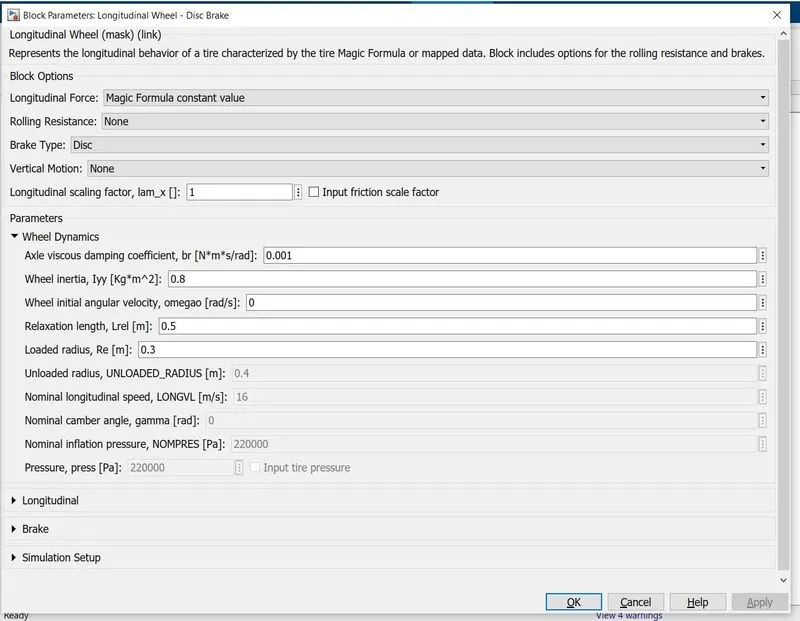
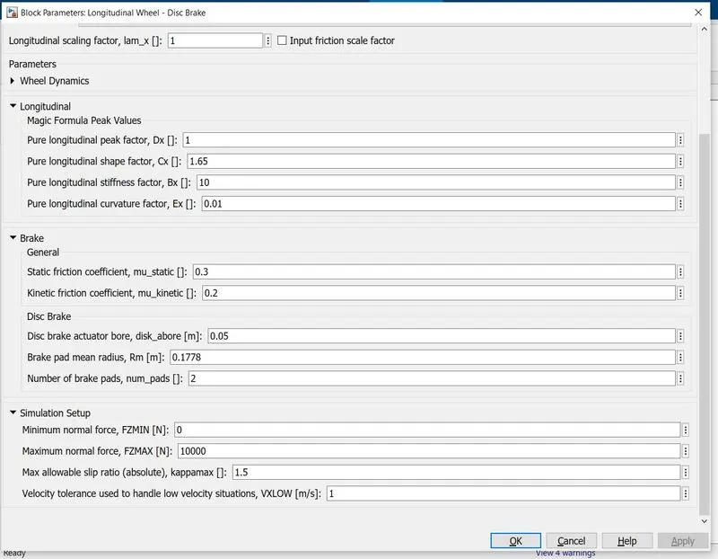
The Longitudinal Wheel block implements the longitudinal behavior of an ideal wheel. You can specify the longitudinal force and rolling resistance calculation method, and brake type. Use the block in driveline and longitudinal vehicle simulations where low frequency tire-road and braking forces are required to determine vehicle acceleration, braking, and wheel-rolling resistance. For example, you can use the block to determine the torque and power requirements for a specified drive cycle or braking event. The block is not suitable for applications that require combined lateral slip.
Ground

Description
The Ground block connects to blocks whose input ports do not connect to other blocks. If you run a simulation with blocks that have unconnected input ports, Simulink® issues warnings. Using a Ground block to ground those unconnected blocks can prevent these warnings.
Working with Fixed-Point Data Types
When working with fixed-point data types, there may be instances where the fixed-point data type cannot represent zero exactly. In these cases, the Ground block outputs a nonzero value that is the closest possible value to zero. This behavior applies only to fixed-point data types with nonzero bias. These expressions are examples of fixed-point data types that cannot represent zero:
-
fixdt(0, 8, 1, 1)— an unsigned 8-bit type with slope of 1 and bias of 1 -
fixdt(1, 8, 6, 3)— a signed 8-bit type with slope of 6 and bias of 3
Working with Enumerated Data Types
When working with enumerated data types, the Ground block outputs the default value of the enumeration. This behavior applies whether:
-
The enumeration can represent zero
-
The default value of the enumeration is zero
If the enumerated type does not have a default value, the Ground block outputs the first enumeration value in the type definition.
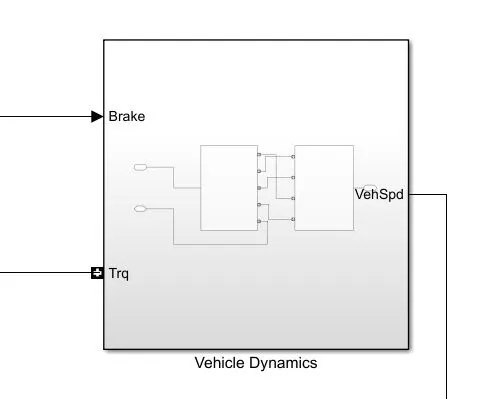
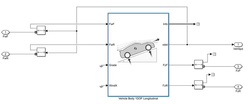
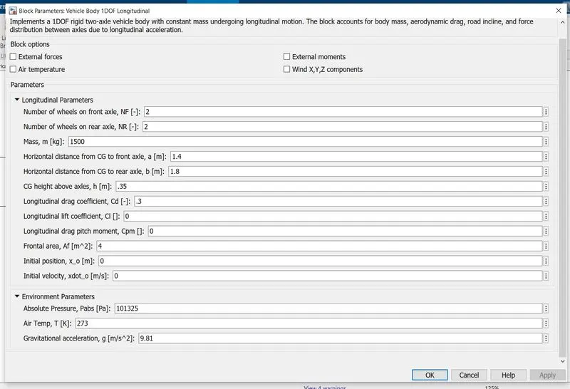
Vehicle Body 1DOF Longitudinal
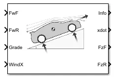
Description
The Vehicle Body 1DOF Longitudinal block implements a one degree-of-freedom (1DOF) rigid vehicle body with constant mass undergoing longitudinal (that is, forward and reverse) motion. Use the block:
-
In powertrain and fuel economy studies to represent the vehicle inertial and drag loads when weight transfer from vertical and pitch motions are negligible.
-
To determine the engine torque and power required for the vehicle to follow a specified drive cycle.
You can select block options to create input ports for external forces, moments, air temperature, and wind speed.
Vehicle Body Model
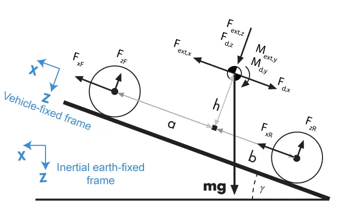
The vehicle axles are parallel and form a plane. The longitudinal direction lies in this plane and is perpendicular to the axles. If the vehicle is traveling on an inclined slope, the normal direction is not parallel to gravity but is always perpendicular to the axle-longitudinal plane.
The block uses the net effect of all the forces and torques acting on it to determine the vehicle motion. The longitudinal tire forces push the vehicle forward or backward. The weight of the vehicle acts through its center of gravity (CG). The grade angle changes the direction of the resolved gravitational force acting on the vehicle CG. Similarly, the block resolves the resistive aerodynamic drag force on the vehicle CM.
Wind and Drag Forces
The block subtracts the wind speeds from the vehicle velocity components to obtain a net relative airspeed. To calculate the drag force and moments acting on the vehicle, the block uses the net relative airspeed.
By default, to calculate the wind speed along the vehicle-fixed x-axis, the block uses the longitudinal wind speed along the earth-fixed X-axis. If you select WindX,Y,Z, the block uses the wind speed along the earth-fixed X-, Y-, Z-axes.
Display
Description
The Display block shows the value of the input data. You can specify the frequency of the display. For numeric input data, you can also specify the format of display.
If the block input is an array, you can resize the block vertically or horizontally to show more than just the first element. If the block input is a vector, the block sequentially adds display fields from left to right and top to bottom. The block displays as many values as possible. A black triangle indicates that the block is not displaying all input array elements.
The Display block shows the first 200 elements of a vector signal and the first 20 rows and 10 columns of a matrix signal.
Displaying Strings
When working with strings, the Display block displays:
-
Strings with double quotes.
-
Special characters such as newline are shown as escaped sequences, for example
'\n'. -
Non-displayable characters as escaped octal number, for example
'\201'.
If the incoming signal is of type string, the Numeric display format parameter selection does not affect the display of the string.
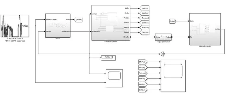
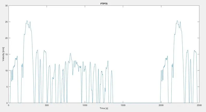
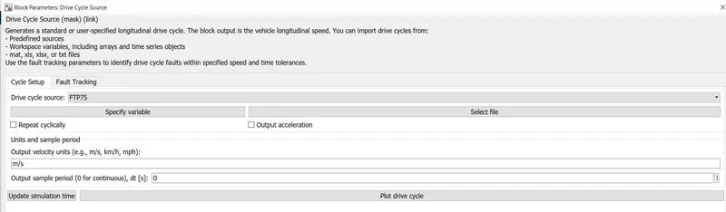
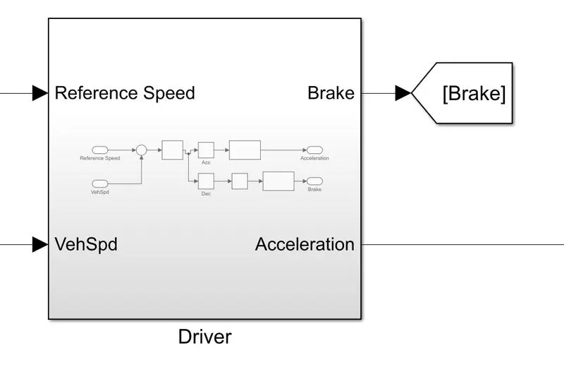
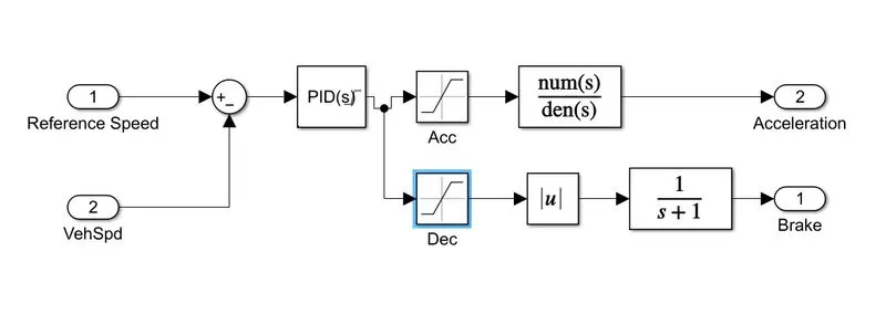
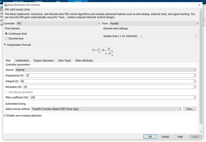
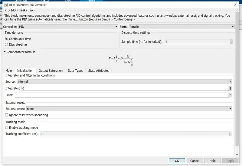
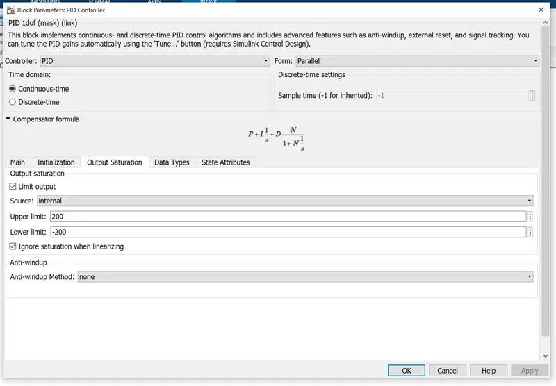
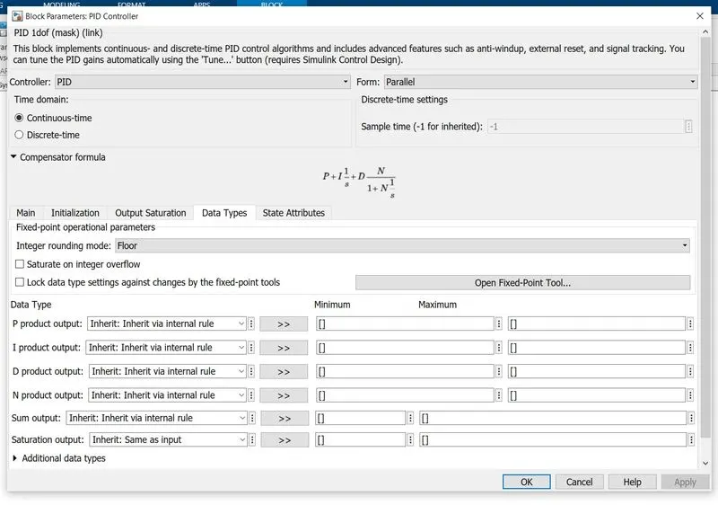
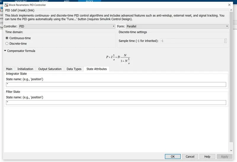
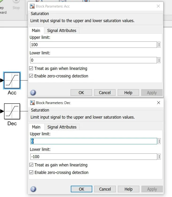
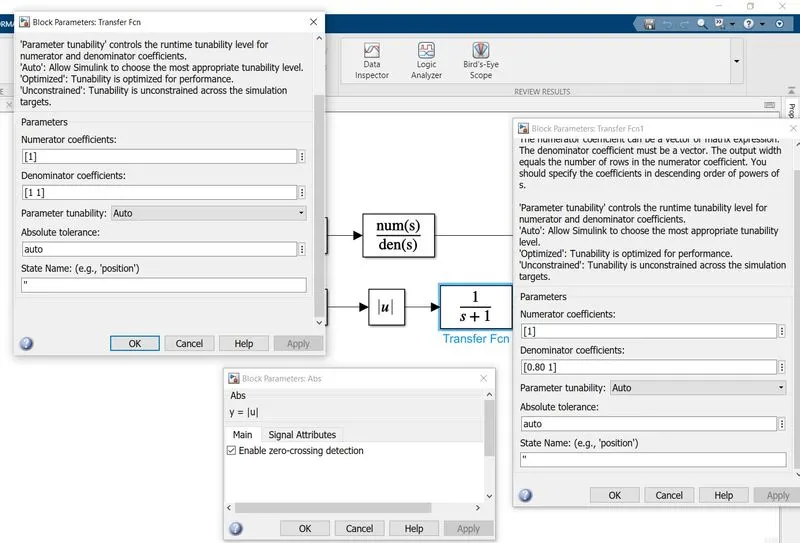
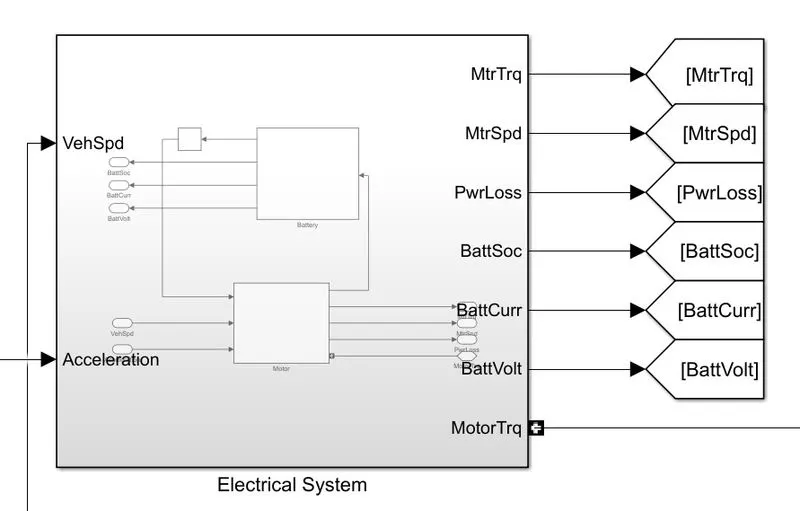
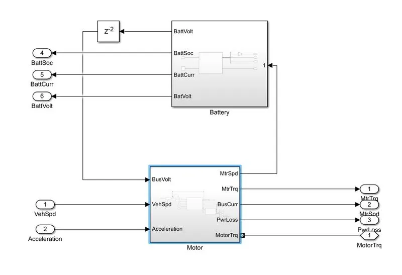
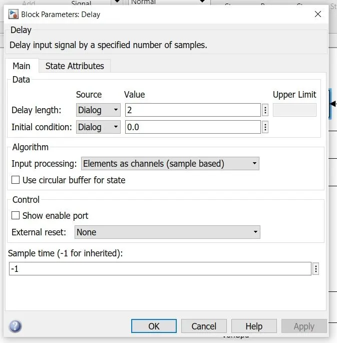
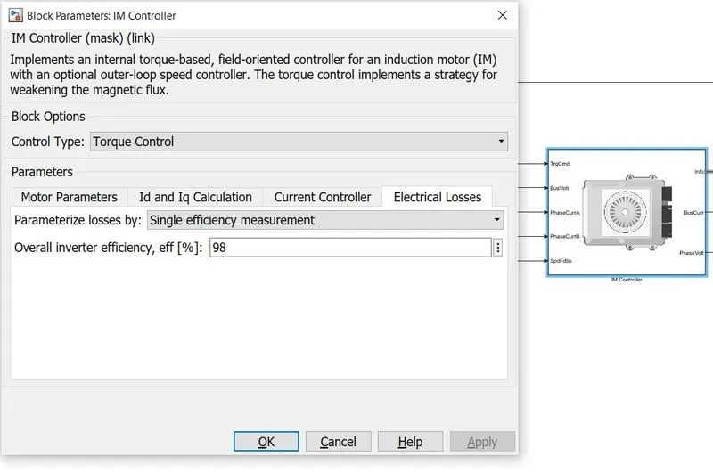
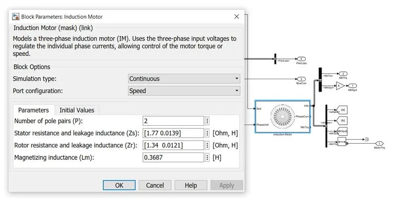
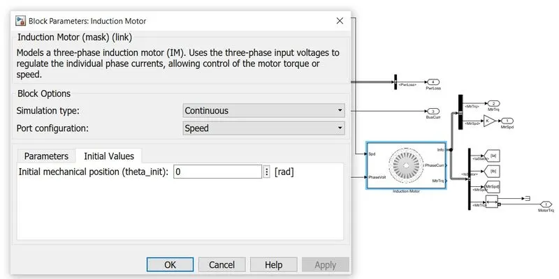
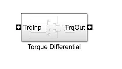
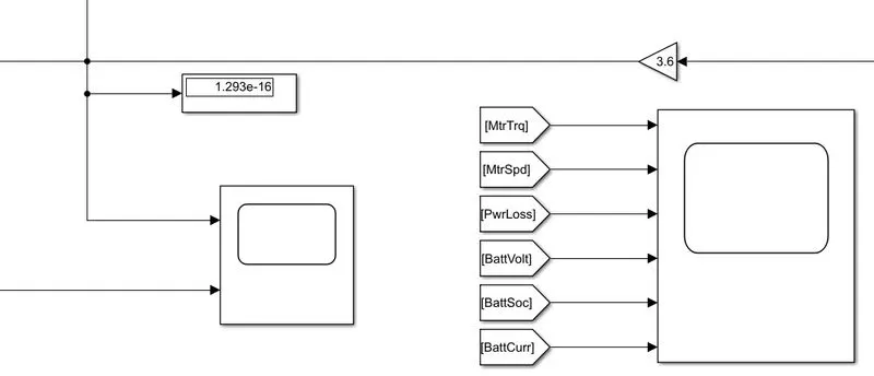
The Following images show the parameters used and also shows the blocks and their connections

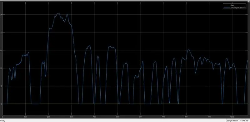
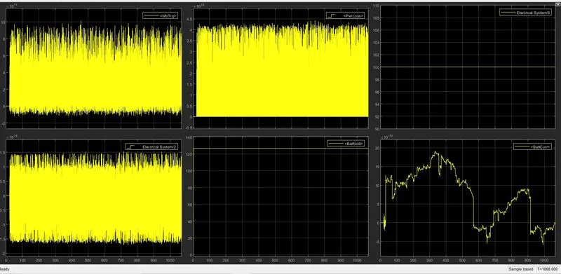
The results are as follows:-