Project-1: Modelling an electric Car with Li-ion battery

Objective: Create a MATLAB model of electric car which uses lithium ion battery and suitable motor. Choose suitable blocks from Simscape or Powertrain block set. Implement the vehicle speed control using PI controller and generate brake and accelerator commands. Avoid using readymade driver block for speed control.

Selecting appropriate parameters of electric vehicle and understanding their characteristics, are the preliminary step in modeling a good electric vehicle. This challenge presents the study of vehicle parameters based on simulation of electric vehicle. All works are performed in MATLAB/Simulink environment.

Keywords: electric vehicle, vehicle parameters, simulation, MATLAB/Simulink.

Theory:

Electric Vehicles (EVs) are vehicles that are powered by electrical energy. The main components of an EV are a motor/generator, motor controller, power converters, wheels, and batteries. The electric motor is used to provide the power required for the wheels to move and provide traction. The motor controller and power converters work together to control the amount of power that is delivered to the motor. The batteries store the electrical energy needed to power the motor.

In this project, I will model an EV in SIMULINK using the powertrain blockset and simscape blocks. This model will implement speed control using a PID controller block. The input to this model will be a Wide Open Throttle (WOT) drive cycle. The output of this model will be blocks that show the total distance travelled by the model and the speed of the vehicle during a 2427 second simulation period. The speed data will reflect both the actual speed of the vehicle and the command speed from the drive cycle data.

To model the EV in SIMULINK, we need to model the individual components of an EV such as the motor, controller, power converters, wheels, and batteries. All of these components are available as blocks from the simscape and powertrain blocksets. The various components of the EV will be modelled and explained in the sections below:

Components of an EV -

An electric powered car has three primary components - Battery, motor controller, and the electric motor.

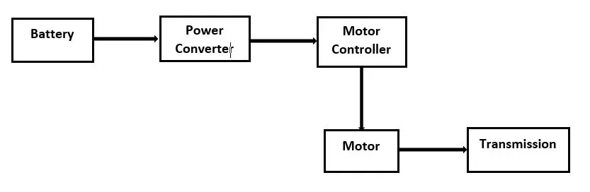
Designing of Electric Motor in Simulink Procedure : While designing we consider the designing in opposite to the flow of power direction .

(1) Vehicle Body Subsystem :

• The vehicle is assumed to be a Rear axle driven (4 wheels - 2 on each axle).
• The wheels are modelled using simple Tire (Magic formula) simulink blocks.
  
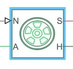
• The N port of the tire corresponds to the Normal Reaction acting on it.
  The A port corresponds to the Mechanical Rotational conserving port for the wheel axle. Thus both the wheels on the same axle should form a connection through their respective A ports.
  Connection H corresponds to the Mechanical Translational conserving port for the wheel hub through which the thrust developed by the tire is applied to the vehicle. Thus, all the 4 wheels form a connection through their respective H ports and this is in turn connected to the translational hub of the vehicle body.
  The connection S represents the output port for slip of the tire.

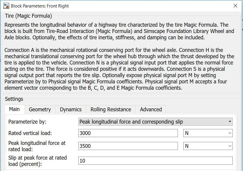
• The tires are parameterized by Peak longitudinal force and corresponding slip.
• The other block parameters such as - rated vertical load, peak longitudinal force at rated load and slip at peak force at rated load - are kept with their default values.

Vehicle Body : This 2 axle (4 wheel) assebly is now connected to a Velocity Body simscape block.

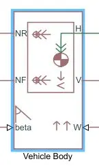
• This block basically represents a two-axle vehicle body in longitudinal motion. The block accounts for -
  body mass,
  aerodynamic drag,
  road incline,
  weight distribution between axles due to acceleration
  road profile.
• Here, the connection H is the mechanical translational conserving port hub.
  NF & NR correspond to the output ports for nomral reaction forces on front axle and rear axle wheels respectively.
  Connection V represents the actual output translational velocity of the vehicle.
  beta is the road inclination angle & W corresponds to the headwind speed (headwind - direction opposite to that of vehicle

• The gross weight is given to be 650 kg.
• The drag force is also considered.

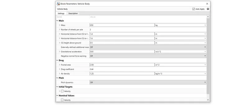
• The pitch dynamics for the vehicle are not considered for this simulation.

The complete Mechanical subsystem is shown below -

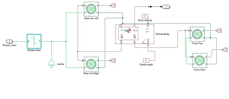
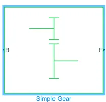
The input for this subsystem is taken as the Rotational speed of the motor. This input is fed to the front axle through a Simple Gear representing the Final Drive Ratio.
Here, the rotational direction of the output shaft is kep the same as that of the input shaft. Also, no meshing losses are considered for the simulation.

(2) DC Motor :

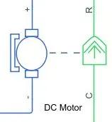
• Simulink provides an inbuilt bodel block for DC motor which converts electrical input into mechanical rotational output.
  Note : Here, the blue colour corresponds to the electrical side of the motor and the green colour corresponds to the mechanical side.
• Here, the motor field type is kept as Permanent magnet and the model parameterization is done by rated load and speed.
  The armature inductance and the mechanical parameters are given their default values.
  All the other parameters are changed as shown below -

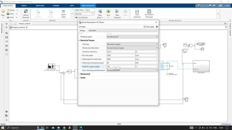
• The connection R represents the Rotor (rotational output) while the connection C is for the Casing (stationary). Thus, the R port is connected to the input of the vehicle subsystem created earlier. The C port is connected to a mechanical rotational reference.
• The + and - terminals of the motor are connected to the motor controller. If these terminals are directly connected to a battery, the required DC motor will run on the rated capacity of the battery. This will eventually result into no control over the DC motor and the vehicle will run at top speed throughout the simulation.
  Thus, a motor controller is very much needed.

Motor Controller :

• H-Bridge circuit -
  
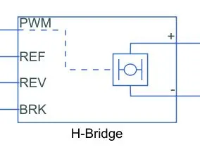
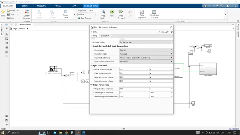
• This block represents an H-bridge motor drive. The block can be driven by the Controlled PWM Voltage block in PWM or Averaged mode.
• In PWM mode, the motor is powered if the PWM port voltage is above the enabled threshold voltage.
• In Averaged mode, the PWM port voltage divided by the PWM signal amplitude parameter defines the ratio of the on-time to the PWM period.
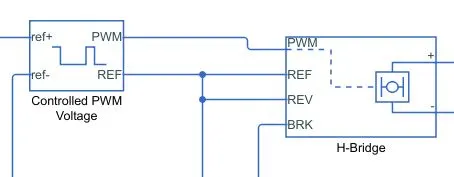
• Connection REF is for the reference input. This combined with the PWM connected will form the pulse input for the H-Bridge.
  Here, the REF input is connected to the Electrical Reference (ground).
• Connection REV corresponds to the reverse motion of the motor which essentially means, the backward motion of the vehicle.
  Here, the backward motion of the vehicle is not accounted for and so, the port is connected to the electrical reference.
• Connection BRK is for the braking of the vehicle.
• Since, the PWM mode results in a huge amount of simulation time, Averaged mode is selected for this simulation.
• Load current characteristics are considered to be smoothed here.
• Also, the regenerative braking depends on REV flag and current sign . This means, when the vehicle starts decelerating, corresponding amount of charge will be fed back to the battery.
  Accordingly, the BRK input is connected to a Controlled Voltage Source. This will generate emf corresponding to the intensity of brakes applied and fed the power back to the battery.

Simulink provides an inbuilt Controlled PWM Voltage block. This block is used for providing the proper pulse inputs to the H-Brdige circuit.

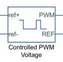
The PWM & REF connections are for the corresponding ports on the H-Bridge circuit.
The 2 reference inputs correspond to the throttle inputs given by the driver. The block generates corresponding pulse width as per the accelerations and brakes apllied by the driver himself.

• Here, the PWM frequency is 1000 Hz. Also, the simulation mode is Averaged as that in the H-Bridge circuit.
  
  
  
  
• The input scaling parameters given are -
  0V for 0% duty cycle and 5V for 100% duty cycle. Accordingly, the output voltage amplitude becomes 5V.

• The H-Bridge circuit along with the PWM input, together form the motor controller circuit.

Battery Pack :

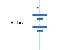
• To model the Battery pack, a simple Battery block is used. This is because, if the generic battery block is used instead, the simulation will run for a much longer time.
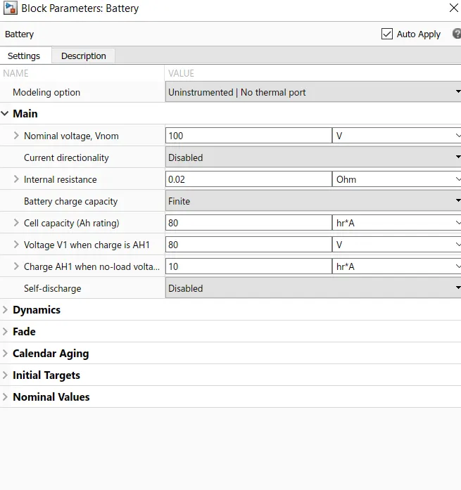
• Here, the selected option for Battery Charge Capacity is Finite. Accordingly, the block models the battery as a series internal resistance plus a charge-dependent voltage source.
  If the chosen option had been Infinite, the voltage source would have been constant.
• Also, the self-discharging of the battery and the battery dynaics are disabled.
• The Battery Nominal Voltage is given as 100V.
  The Ampere-hour rating is assumed to be 80.
  The rest all paramaters are left with their default values.

To ensure the battery supplies current as per the requirements of the motor controller and not the rated current, a Current Sensor & Controlled Current Source pair is connected.

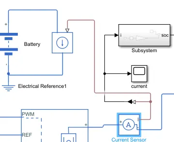
(7) Battery State of Charge :

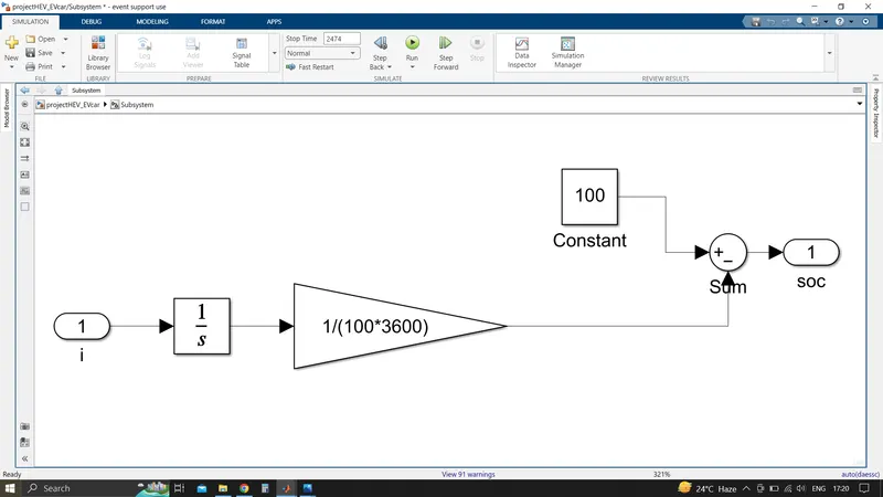
• A small subsystem is created to calculate the State of Charge of the battery.
• This subsystem takes the battery current as the input.

• The essential process to calculate the SOC is by subtracting the charge from the rated capacity of the battery.
• Accordingly, the current is integrated w.r.t. time to get the charge in coulumbs. Now this coulumb value is modified into Ampere hours.
  This value is now subtracted from the charging capacity of the battery i.e. 100 Ah.
• Finally, the remaining charge is now converted into percentage value of the charging capacity of the battery.

Reference Velocity (Drive Cycle) :

• The Drive Cycle Source block is used to provide the reference speed for the simulation.
• It generates a standard or user-specified longitudinal drive cycle.
  
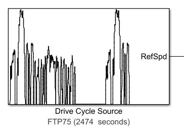
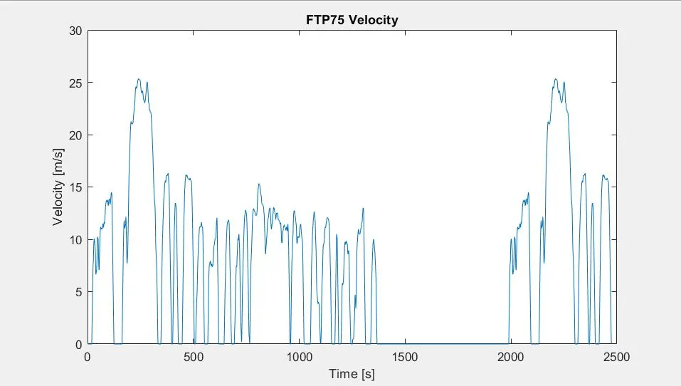
• Here, the selected drive cycle is the standard FTP75.
  
  
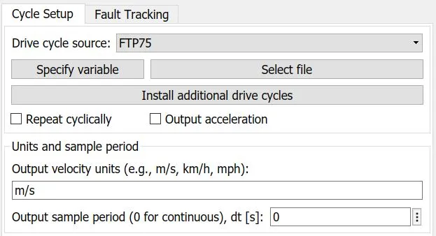
• The plot of the drive cycle is shown below -
  
  

Simulation :

• The system is run for simulation for 2474 s which is the total time for which the input drive cycle is defined.
• A Solver Configuration is added to ensure proper solving of the mathematical equations by the model.
• The simscape solver
  
• Scopes are connected to analyze different outputs such as the SOC of the battery, the reference velocity & the actual velocity of the vehicle and the distance covered by the vehicle during the total run.
• The 2 velocities are first converted from m/s to kmph values. For this, simple Gain blocks are used.
• The distance is calculated by simply time-integration of the vehicle velocity.

Sum Block

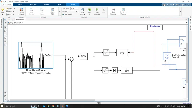
The "Sum" block is used as part of a feedback system. This system will require data from the drive cycle (command signals) and data from the vehicle body (actual speed) as well. The aim of this speed control system is to have the actual vehicle speed to match the command speed data from the drive cycle as closely as possible. The feedback system is essential to this control method because it will relay the actual speed data back for a comparison with the drive cycle data. Any difference in the data between the two is considered as an error and the sum block is used to find the difference.

This block is shown below:

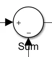
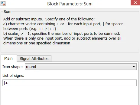
In order to find the difference between the drive cycle data and the actual speed from the vehicle block, the list of signs need to be changed to "+-".

PID Controller

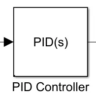
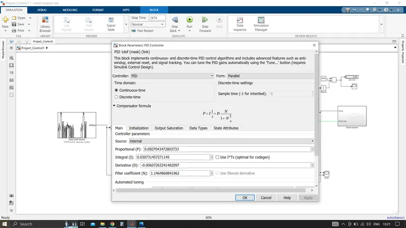
The PID controller block is essential for the speed control of the EV model. The PID controller block takes the error data between the drive cycle data and the actual speed of the vehicle (from the sum block) and works to minimize this error. The PID controller block is shown below:

Saturation Block

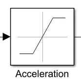
In order to set the acceleration and brake commands, I have used the saturation block. This block is used when we want to set limits for signals. This block is shown below:

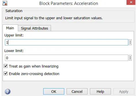
In the case of the accelerator command, I have set the limits between 0 and 1 by opening the saturation block parameters as shown below:

Another saturation block was used for the deceleration/brake commands which is shown below:

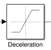
To create the deceleration commands, I have used a different set of limits between -1 and 0. This is shown in the image below:

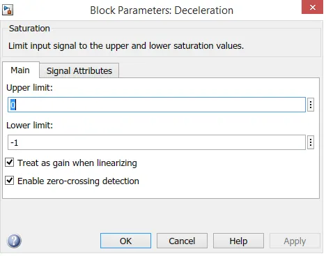
These limits ensure that there is no crossover with the acceleration commands.

Transfer Function

The transfer function block is used when we want to insert a transfer function. A transfer function is defined as the ratio of the Laplace transform of the output of a system to the input of a system. The transfer function block is shown below:

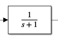
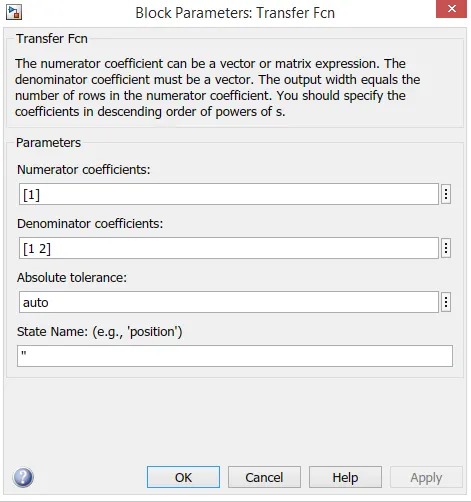
Double-clicking the block opens the block parameters as shown below:

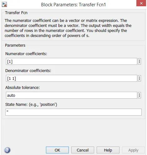
From the block parameters, we can modify the transfer function by changing the numerator and denominator coefficients. I have used the default coefficients.

For the deceleration command, I have used another transfer function block with a slightly different transfer function. This is shown in the image below:

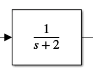
The transfer function block was modified by changing the coefficient of the denominator as shown in the image below:

Absolute Block

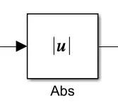
An absolute block is also implemented for the deceleration command which takes the absolute value from the deceleration saturation block. This block is shown below:

Speed Measurement

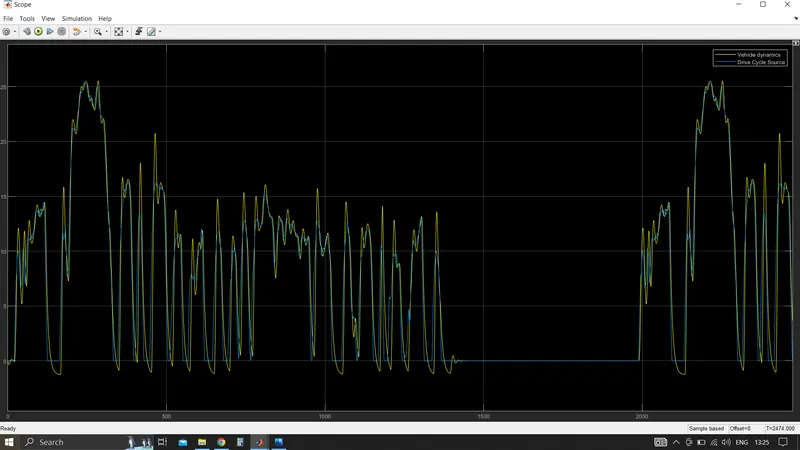
In order to measure the speed of the EV model, I needed to use the scope block once again. I modified the scope block to have 2 input ports where one port takes the output velocity signal from the vehicle subsystem block and the other port takes the output signal from the drive cycle to the reference velocity port on the longitudinal driver block. This has been done so that the scope can show us the plots of the reference velocity and the actual velocity of the vehicle to see how they compare with each other.

Distance Measurement

I have used the scope block and mathematical operator blocks to measure the distance travelled by the vehicle according to the drive cycle data. The area under a velocity time graph tells us the distance travelled by an object and so in my model. This means that the integral of the velocity with respect to time, gives us the distance travelled. So, I have implemented the integrator block to integrate the velocity signal that is output from the vehicle subsystem.

The integrator block is shown below:

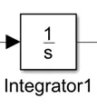
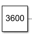
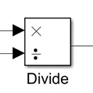
From the integrator block, I needed to use the 'Divide' block along with a 'Constant' block having a value of 3600 in order to convert the divide the integrated speed signal which is in kilometres per hour by 3600. This will give us the distance travelled in kilometres.

The constant block with a value of 3600:

The 'Divide' block:

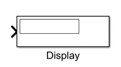
Finally, a 'Display' block is used to show the distance travelled as the simulation is run. The display block is shown below:

Model:

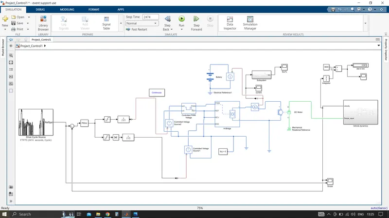
Scope Result Tunned :

Conclusion : Hence We could achive Reference speed at some more extend after performing tunning with PID controller. Because this plant is not the linear model so we have to use the linearization method to tune the model .