Project-1: Modelling an electric Car with Li-ion battery

An electric car is powered by an electric motor instead of a petrol engine. The electric motor gets energy from a controller, which regulates the amount of power—based on the driver’s use of an accelerator pedal. The electric car (also known as an electric vehicle or EV) uses energy stored in its rechargeable batteries, which are recharged by common household electricity.

Thus an electric vehicle will have three basic components :

• Energy Storage Unit
• Controller
• Propulsion system

The energy storage unit will have a way to store power. A chemical battery is the most common energy storage technology currently, although it can be different - for example - A fuel cell (which gets its electricity from hydrogen rather than a battery pack), can be used instead of a chemical battery as the energy storage unit.
The controller acts as a pipeline or gateway to the electric motor.. The controller will do other things too - it moderates the power, will also act as a converter - converts power from DC to AC, or it might also increase or decrease the amperage etc. The controller is the brains of the system.
The electric motor, which is the propulsion system, converts the electric power and converts this into physical energy for movement.

The whole system is a much simpler, more efficient device than the combustion engine found in most cars, enabling you to get the most mileage for your charge.

Historically, EVs have not been widely adopted because of limited driving range before needing to be recharged, long recharging times, and a lack of commitment by automakers to produce and market electric cars that have all the creature comforts of petrol-powered cars. That’s changing. As battery technology improves—simultaneously increasing energy storage and reducing cost—major automakers are expected to begin introducing a new generation of electric cars.

Electric cars produce no tailpipe emissions, reduce our dependency on oil, and are cheaper to operate. Of course, the process of producing the electricity moves the emissions further upstream to the utility company’s smokestack—but even dirty electricity used in electric cars usually reduces our collective carbon footprint.

Another factor is convenience - Let's not forget two important points: charging up at home means never going to a petrol station—and electric cars require almost none of the maintenance, like oil changes and emissions checks, that internal combustion cars require.

Electric motors develop their highest torque from zero RPMs—meaning fast (and silent) zero-to-60 acceleration times.

To model the EV in SIMULINK, we need to model the individual components of an EV such as the motor, controller, power converters, wheels, and batteries. All of these components are available as blocks from the simscape and powertrain blocksets. The various components of the EV will be modelled and explained in the sections below:

Vehicle Body

To model the body of the EV, we need to insert the vehicle body block shown in the image below:

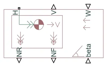
This block has 6 ports which represent various aspects of the modelling of the vehicle body:

• H - This stands for hub and allows us to connect the hubs of the wheels of the vehicle to the body.
• V - This stands for velocity and outputs the velocity of the vehicle.
• W - This represents wind velocity and allows us to model a headwind (against the front of the vehicle) acting on the velocity by giving a speed for it.
• NR - This represents the normal force on the rear wheels of the vehicle.
• NF - This represents the normal force on the front wheels of the vehicle.
• beta - This represents the grade (incline) of the surface that the vehicle travels on, as an angle to the horizontal.

Double-clicking the vehicle body block opens the block parameters shown below:

parameters:

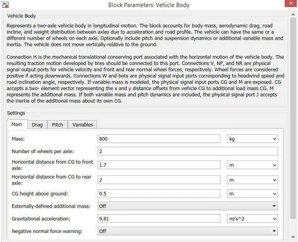
From the "Main" tab, here, we can model the basic parameters of the vehicle such as mass, number of wheels per axle, and even gravitational acceleration. For our model, we are using a mass of 800kg, 2 wheels per axle (total of 4 wheels), and gravitational acceleration of 9.81 meters per second squared.

Drag Tab

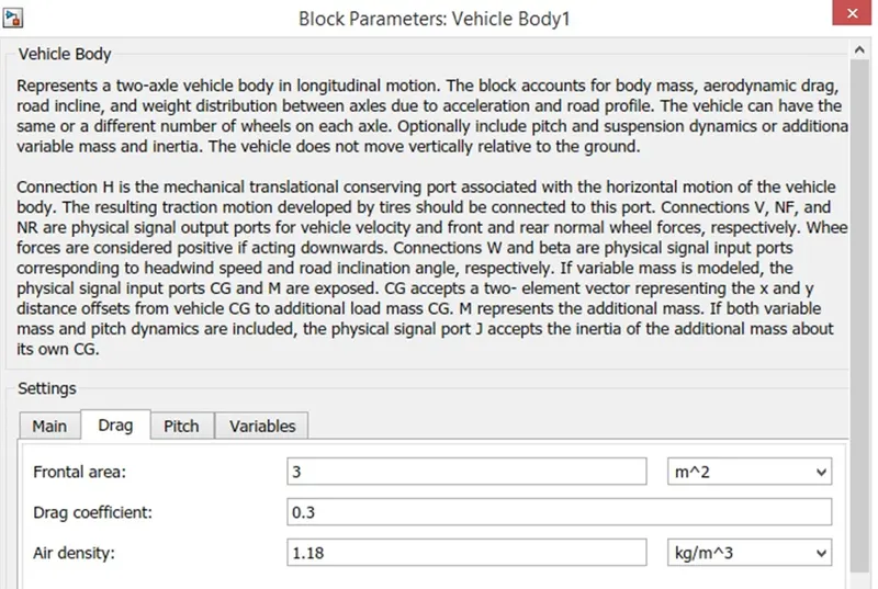
From the "Drag" tab, we can model the frontal area, drag coefficient, and the air density. I have used a frontal area, drag coefficient, and air density of 3, 0.3, and 1.18 respectively.

Wind Velocity & Slope

From the "W" and "beta" ports on the vehicle body block, I have used a "PS-Constant" block to model the effect of the wind velocity and the slope.

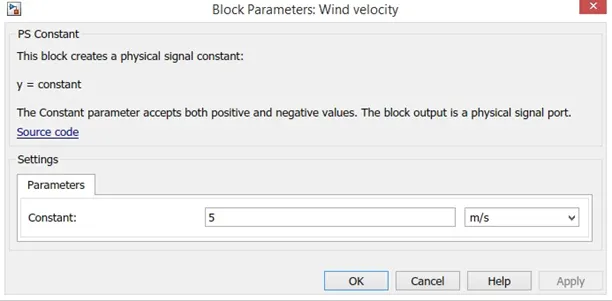
For the wind velocity, I have used a constant value of 5.

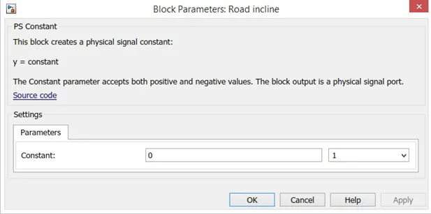
For the road incline, I have used a constant value of 0.

Tires

In this model, I have used the "Magic Formula" tires. There are various tire blocks that can be used, but the advantage of the magic formula ones is that they enable us to model the longitudinal behavior of tires on a highway. This block is shown below:

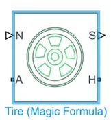
This block has 4 ports which represent various factors that can be modelled:

• N - This port represents the normal force on the tire and the downward direction is considered positive.
• S- This port represents the slip acting on the tire.
• A - This port represents the axle and is the mechanical rotational conserving port for the wheel axle.
• H - This port represents the hub and is the mechanical translational conserving port for the wheel hub.

Double-clicking the magic formula tire block, opens the block parameters window shown below:

parameters:

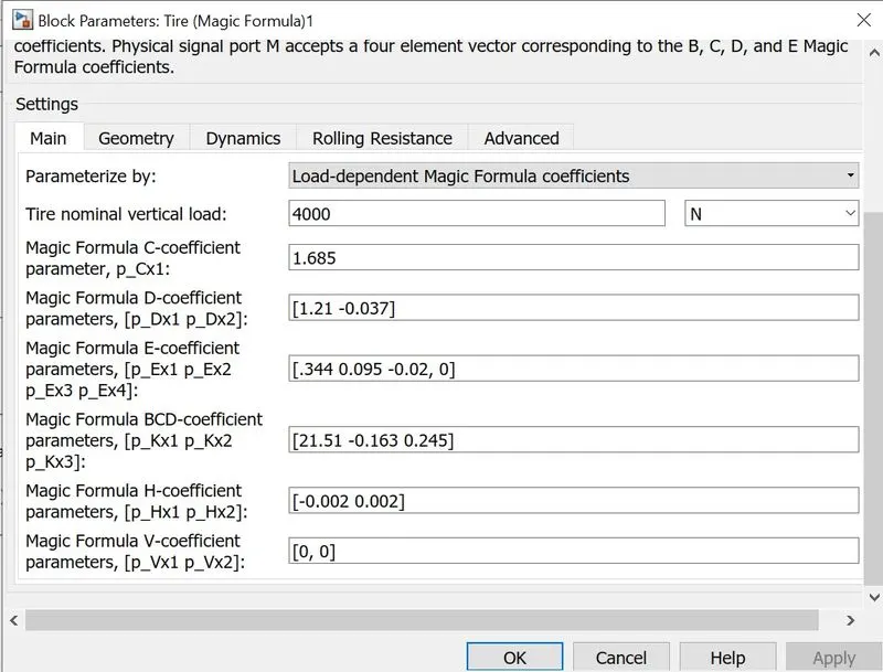
In the "Main" tab, we can model parameters such as tire nominal vertical load, and various coefficients. All values are kept as default.

Gear

In this section, I have modelled the transmission of the EV. To simplify the transmission system of the EV model, I have used a "Simple Gear" block which uses a fixed gear ratio with no inertial effects. This block is shown below:

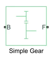
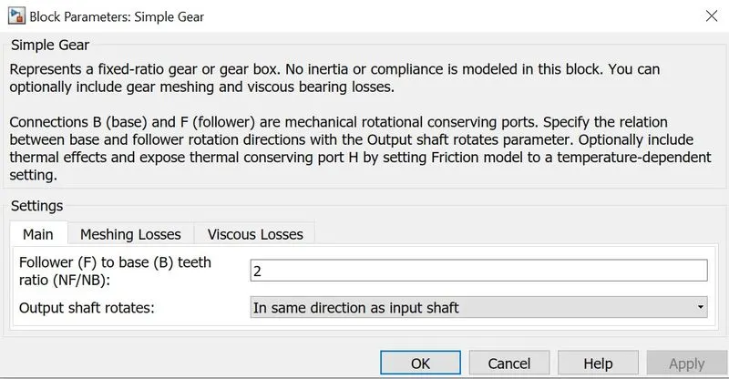
Double-clicking this block, opens the block parameters where we can model additional parameters of the gear.

parameters:

Side Shaft

The side shaft block is used to create inertial effects on the simple gear. This block only has one mechanical rotational conserving port and the positive direction of the block is from the port to the reference point (simple gear block). The side shaft block is shown below:

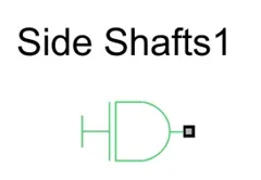
Double-clicking the side shaft block, opens the side shaft block parameters shown below:

Parameters:

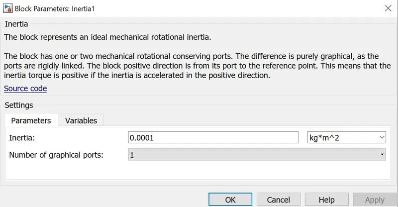
In the "Parameters" tab, we can model the inertia of the side shaft. The default value of 0.0001 is used.

Vehicle Body Subsystem:

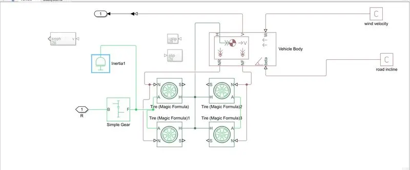
The full vehicle body system is shown in the image above with all the aforementioned blocks connected together. Four magic tire block are used to represent a four-wheeled vehicle.

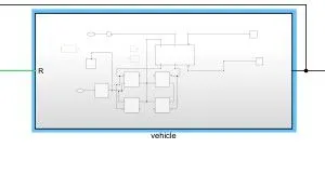
This system is then converted to a subsystem shown in the image below:

Motor

For our EV model, I am using a DC motor block which is shown below:

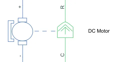
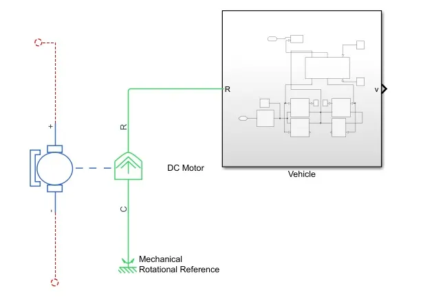
The left side of the motor represents the electrical part of the motor, whereas the right side represents the mechanical part. The mechanical part has 2 ports labelled C and R. C refers to the casing of the motor and R represents the rotation of the motor which produces the torque. The electrical part has 2 ends labelled with a positive and negative sign which represent the positive and negative terminals of the motor.

Double-clicking the motor block opens the block parameters:

parameters:

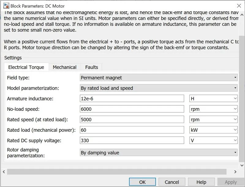
Under the "Electrical Torque" tab, we can model the electrical torque characteristics of the DC motor such as no-load speed, and rated DC supply voltage. I have used the values and settings shown in the image above.

Mechanical

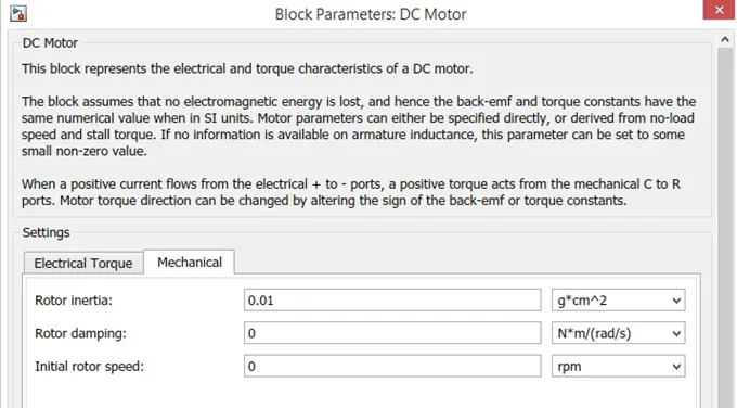
Under the "Mechanical" tab, we can model the mechanical torque characteristics such as rotor inertia and initial rotor speed. I have used the default values as shown in the image above.

After setting the DC motor block parameters, make the connections as given in the image below:

H-Bridge Motor Driver

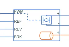
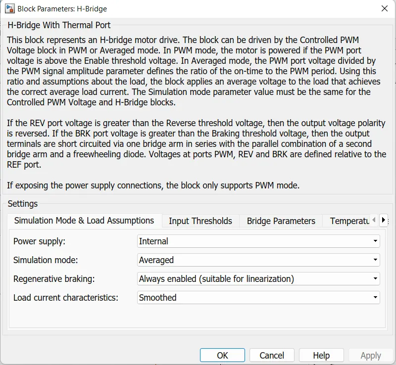
The H - Bridge with Thermal Port block is used to drive a motor. The H bridge two output ports

Positive Port

Negative Port

This port is directly connected to the motor that has to be controller. There is also a REV port.When the reverse threshold voltage is lower than the REV port voltage,the polariy of the motor is reversed, and if the BRK port voltage is greater than the value of breaking threshold voltage, it indicates that the vehicle is in braking condition.

The following image shows the H-Bridge Motor Driver block from Powertrain block set.

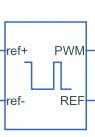
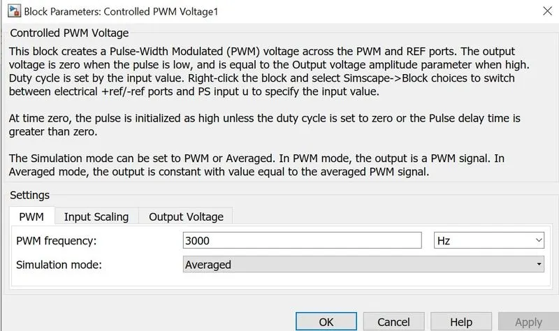
Controlled PWM Voltage Source

The PWM signal is used or controlling the speed of the traction motor. This block is used for providing a controlled PWM voltage output.

The Duty cycle is given by,

100*(Vref-Vmin/Vmax-Vmin)

Where,

Vref - is the reference voltage across the ref+ and ref- ports.

Vmin - denotes the minimum reference voltage.

Vmax - denotes the minimum reference voltage.

The following image shows the Controlled PWM Voltage Source block from Powertrain blockset.

Current Sensor

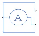
This block is used to measure the flow current through of circuit.

Controlled voltage Source

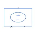
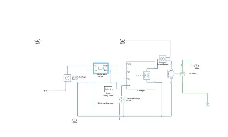
The controlled voltage source block is used to give a constant voltage output. It has two electrical conserving ports and a physical signal port. The output from the controlled voltage source is fed to the controlled PWM voltage source.

Electrical Reference

The electrical reference block is used to create a grounding effect for electrical circuits. Any model that uses electrical or electronics components will need to have atleast one electrical reference block in it. The electrical reference block is shown below:

In this EV model, we are using this block for 2 occasions. The first is for to create an electrical ground between the controlled voltage source, controlled PWM voltage and the H-Bridge blocks. The second is for the battery system which will be modelled afterwards,

Solver Configuration

The solver configuration block is used to solve any necessary equations in a model and in my case, I have used them in the connection to the 'REV' port of the H-Bridge block. The solver configuration block is shown below:

The image below shows the connections that can be made with the components discussed till this point.

Battery And Soc Subsystem Model:

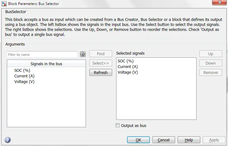
Battery

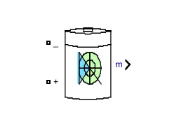
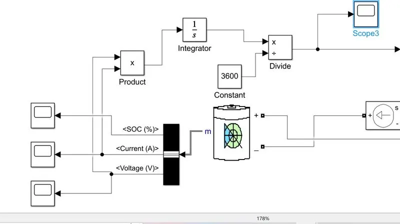
• The battery is required to power the controller and motor. The controller uses the battery power according to produce the input given by the motor to obtain maximum speed. The battery is also used to power every electrical component in the vehicle.
• The Battery block implements a generic dynamic model that represents most popular types of rechargeable batteries.

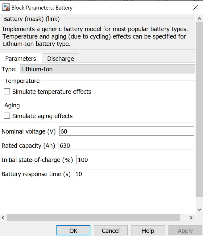
The battery has two stages one is charging and other one is discharging state. The battery is of 75Ah capacity.
Initial SoC is 100%

Drive Cycle:

A drive cycle is a data set that contains velocity and time data for the purpose of modelling the motion of a vehicle. The drive cycle will be a plot of the velocity against the time and it is made to resemble typical driving conditions that a consumer may experience themselves in. For instance, they can model highway driving situations, driving in urban areas, or driving with full power etc. Drive cycles are used by automotive companies for various testing procedures such as mileage, pollution tests, and acceleration and top speed tests. There are various different drive cycles that are industry standard e.g. Urban Dynamometer Driving Schedule (UDDS), FTP 75.

In my EV model, a drive cycle is used as the reference velocity data for the longitudinal driver block to send acceleration or deceleration commands according to the drive cycle. There are 3 ways of implementing a drive cycle. One method is to create or own drive cycle with a spreadsheet of velocity data in one column and time data in another column. Another method is to use a signal builder block and create signals that represent the velocities at which the vehicle should travel and the durations for which those velocities are to be maintained. The last method is to use the industry standard drive cycles which are in - built in to the SIMULINK library. In my case, I have used an industry standard 'WOT' drive cycle. This drive cycle stands for 'Wide Open Throttle' and it models the situation where the vehicle is made to accelerate at full power and maintained at a particular speed and made to decelerate back to rest.

By default, the drive cycle block is set to the FTP75 drive cycle shown below:

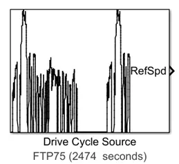
This can be modified by opening the block parameters shown below:

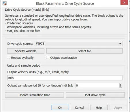
When the 'WOT' drive cycle is chosen, some extra parameters are made available for modification which are shown below:

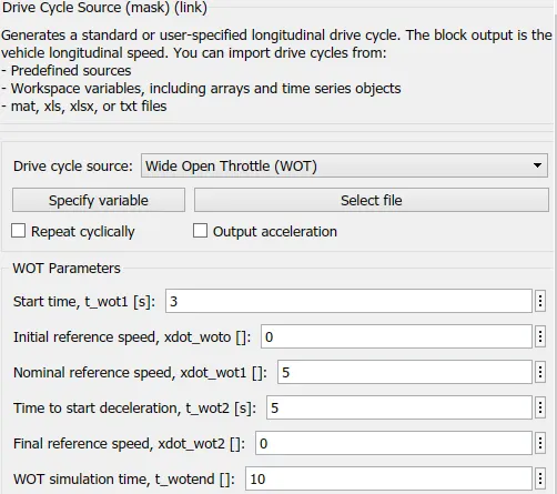
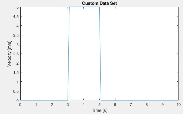
As we can see, with the 'WOT' drive cycle, we can modify the start time, time to start deceleration, and the entire duration of the drive cycle. I have used a start time of 3 seconds meaning that the vehicle will begin acceleration after 3 seconds of starting simulation. I have used a nominal reference speed of 5 m/s and this refers to the maximum speed the vehicle should achieve. I have set the deceleration to begin at t = 5 seconds and the whole cycle is set for a duration of 10 seconds. The input and output velocity units are both set to m/s.

The plot below shows the custom WOT drive cycle I have created.

Sum Block

The "Sum" block is used as part of a feedback system. This system will require data from the drive cycle (command signals) and data from the vehicle body (actual speed) as well. The aim of this speed control system is to have the actual vehicle speed to match the command speed data from the drive cycle as closely as possible. The feedback system is essential to this control method because it will relay the actual speed data back for a comparison with the drive cycle data. Any difference in the data between the two is considered as an error and the sum block is used to find the difference.

This block is shown below:

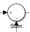
Double-clicking the sum block opens the block parameters as shown below:

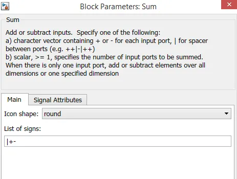
In order to find the difference between the drive cycle data and the actual speed from the vehicle block, the list of signs need to be changed to "+-".

PID Controller

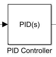
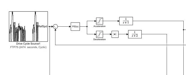
The PID controller block is essential for the speed control of the EV model. The PID controller block takes the error data between the drive cycle data and the actual speed of the vehicle (from the sum block) and works to minimize this error. The PID controller block is shown below:

Double-clicking the block opens the block parameters shown below:

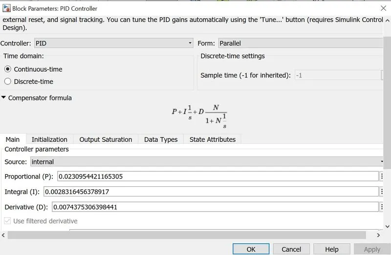
In this model, I have used the continuous-time domain PID controller. All other parameters are left as default.

Saturation Block

In order to set the acceleration and brake commands, I have used the saturation block. This block is used when we want to set limits for signals. This block is shown below:

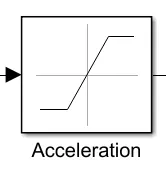
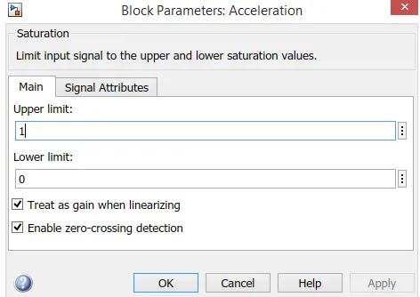
In the case of the accelerator command, I have set the limits between 0 and 1 by opening the saturation block parameters as shown below:

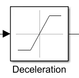
Another saturation block was used for the deceleration/brake commands which is shown below:

To create the deceleration commands, I have used a different set of limits between -1 and 0. This is shown in the image below:

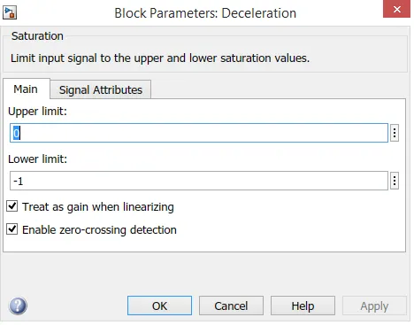
These limits ensure that there is no crossover with the acceleration commands.

Transfer Function

The transfer function block is used when we want to insert a transfer function. A transfer function is defined as the ratio of the Laplace transform of the output of a system to the input of a system. The transfer function block is shown below:

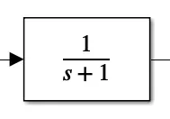
Double-clicking the block opens the block parameters as shown below:

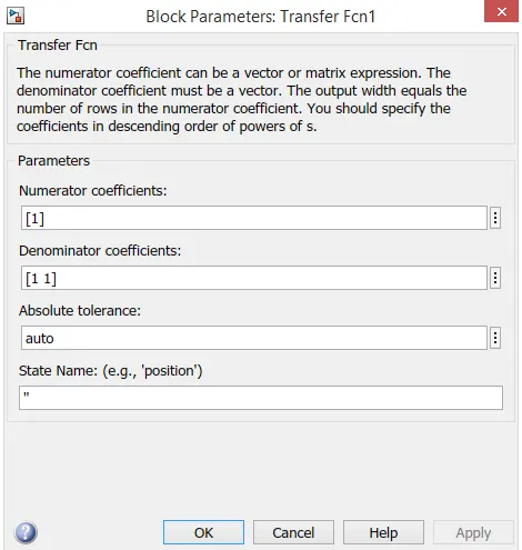
From the block parameters, we can modify the transfer function by changing the numerator and denominator coefficients. I have used the default coefficients.

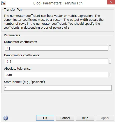
For the deceleration command, I have used another transfer function block with a slightly different transfer function. This is shown in the image below:

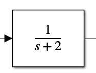
The transfer function block was modified by changing the coefficient of the denominator as shown in the image below:

Absolute Block

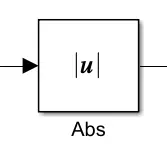
An absolute block is also implemented for the deceleration command which takes the absolute value from the deceleration saturation block. This block is shown below:

With the aforementioned blocks, the control system can be made as shown in the image below:

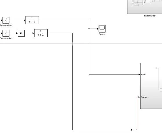
The accelerator and brake commands can be connected to the power converter as shown in the image below:

Speed Measurement

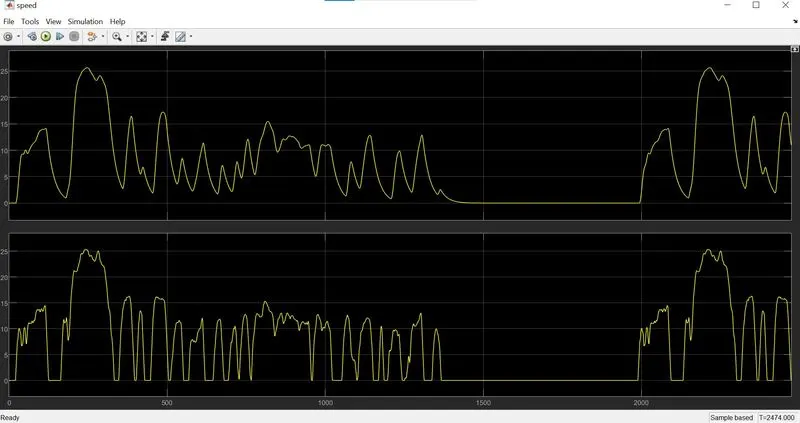
In order to measure the speed of the EV model, I needed to use the scope block once again. I modified the scope block to have 2 input ports where one port takes the output velocity signal from the vehicle subsystem block and the other port takes the output signal from the drive cycle to the reference velocity port on the longitudinal driver block. This has been done so that the scope can show us the plots of the reference velocity and the actual velocity of the vehicle to see how they compare with each other.

Distance Measurement

I have used the scope block and mathematical operator blocks to measure the distance travelled by the vehicle according to the drive cycle data. The area under a velocity time graph tells us the distance travelled by an object and so in my model. This means that the integral of the velocity with respect to time, gives us the distance travelled. So, I have implemented the integrator block to integrate the velocity signal that is output from the vehicle subsystem.

The integrator block is shown below:

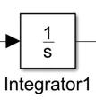
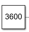
From the integrator block, I needed to use the 'Divide' block along with a 'Constant' block having a value of 3600 in order to convert the divide the integrated speed signal which is in kilometres per hour by 3600. This will give us the distance travelled in kilometres.

The constant block with a value of 3600:

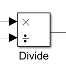
The 'Divide' block:

Finally, a 'Display' block is used to show the distance travelled as the simulation is run. The display block is shown below:

If these blocks have been added to the workspace, they can be connected as shown in the image below:

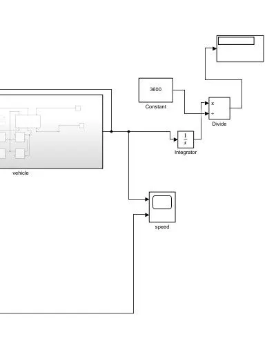
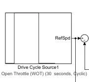
From the drive cycle block, a connection is given to the speed scope block to plot the drive cycle data during the simulation. From the speed scope block, a connection is sent back to the control system to the sum block negative port for the feedback control to occur.

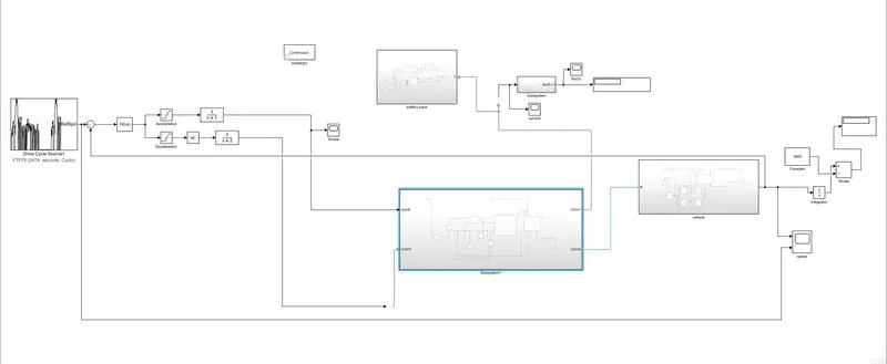
Model:

Result:

After running this model using the FTP75 drive cycle and tuning the pid blocks values as shown in below:

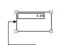
4.94kmps distance covered by the vehicle in the FTP75 drive cycle.

For the same simulation time, the following PID values were used:

• K_i =0.0028316456378917
• K_p =0.0230954421165305
• K_d = 0.0074375306398441

For these PID values, the following speed-time plot was obtained:

Scope:

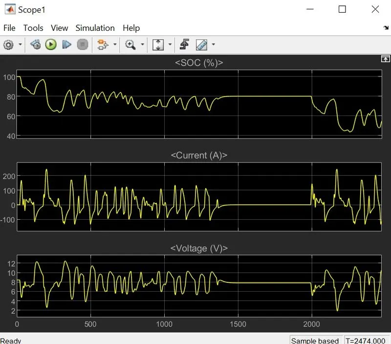
I change the drive cycle and set the Wide open throttle WOT drive cycle and set the simulation time as the 30s and run the module result as shown below.

Result:

Distance:

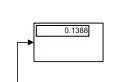
0.1388kmps distance covered by the vehicle in WOT drive cycle.

Scope:

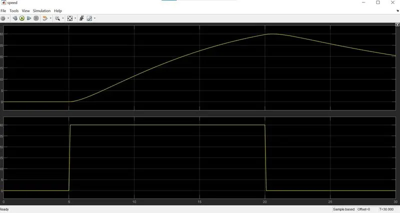
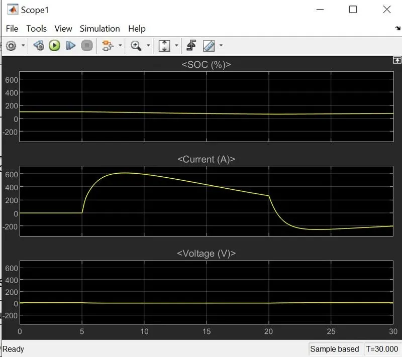
In this attempt, the overall speed behavior of the vehicle is unchanged. However, the peak speed was the highest compared to all other simulation attempts. There is still a delayed response time in the acceleration of the vehicle and the vehicle fails to achieve the commanded peak speed of 5 m/s. The vehicle also fails to maintain the actual peak speed for the commanded 2 seconds of time.

Conclusion:

The Matlab model of an Electric Vehicle has been successfully made by choosing Suitable blocks from the powertrain block set. We understand how to make the model of an Electric Vehicle by using powertrain blocks.