Project 1 - Data Handling and Interpolation
1.
% Input Dialog for Parameters
answer = inputdlg({'Mass (m)', 'Spring Constant (k)'}, 'Input Parameters', 1, {'0', '0'});
m = str2double(answer{1});
k = str2double(answer{2});
% Define ODE
oscillator = @(t, y) [y(2); -k/m * y(1)];
initial_conditions = [1; 0];
tspan = [0 10];
% ode45
[t45, y45] = ode45(oscillator, tspan, initial_conditions);
% ode23
[t23, y23] = ode23(oscillator, tspan, initial_conditions);
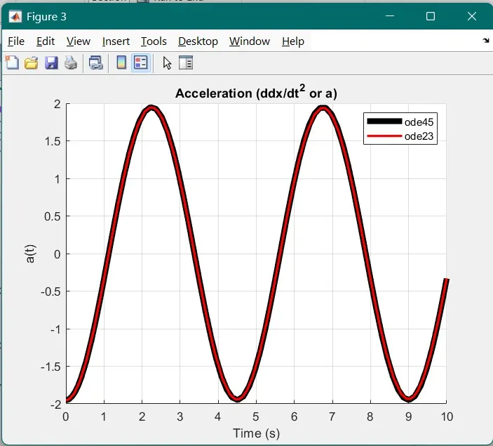
% Calculate Acceleration
acceleration45 = -k/m * y45(:,1);
acceleration23 = -k/m * y23(:,1);
% Plot
figure;
subplot(3,1,1);
plot(t45, y45(:,1), 'r', t23, y23(:,1), 'b');
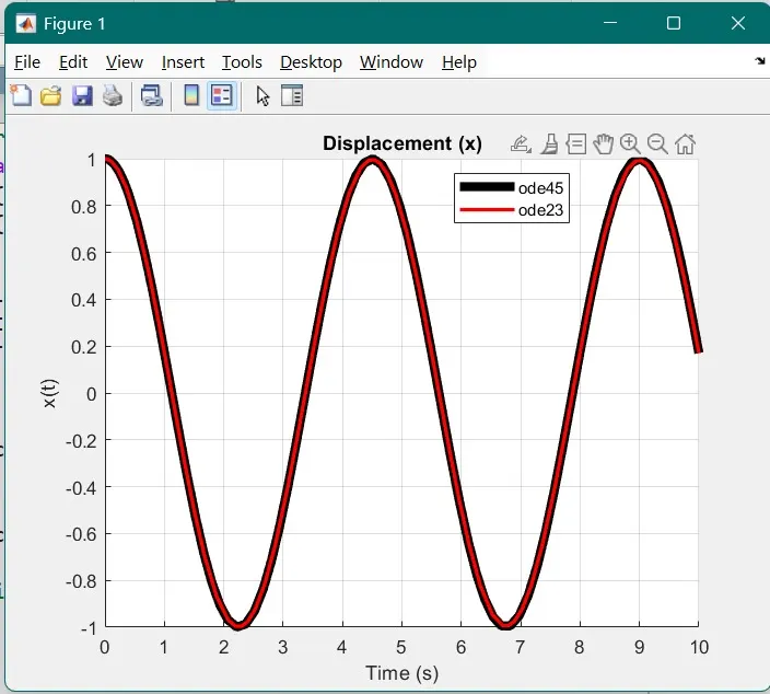
title('Displacement (s)'); legend('ode45', 'ode23');
subplot(3,1,2);
plot(t45, y45(:,2), 'r', t23, y23(:,2), 'b');
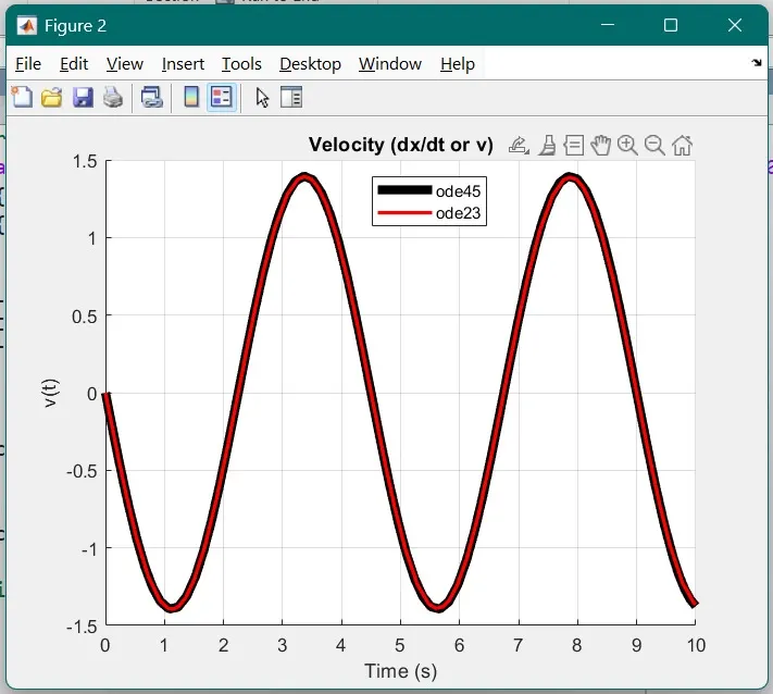
title('Velocity (v)'); legend('ode45', 'ode23');
subplot(3,1,3);
plot(t45, acceleration45, 'r', t23, acceleration23, 'b');
title('Acceleration (a)'); legend('ode45', 'ode23');
2.
% Load Data
data = readmatrix('altitude_temperature_data.csv');
% Extract Altitude and Temperature
altitude = data(:, 1);
temperature = data(:, 2);
% Fit and Evaluate Polynomial Regression
%polynomial degree
degree = 2;
p = polyfit(altitude, temperature, degree);
evaluated_temp = polyval(p, altitude);
% Plot Results
plot(altitude, temperature, 'o', altitude, evaluated_temp, '-');
title('Altitude vs Temperature');
xlabel('Altitude (m)'); ylabel('Temperature (°C)');
legend('Original Data', 'Fitted Curve');
grid on;
% Save Evaluated Data
writematrix([altitude, evaluated_temp], 'evaluated_data.txt', 'Delimiter', '\t');
disp('Evaluated data saved to "evaluated_data.txt".');
3.
% Load Data
data = readmatrix('altitude_temperature_data.csv');
% Extract Altitude and Temperature
altitude = data(:, 1);
temperature = data(:, 2);
% Fit and Evaluate Polynomial Regression
%polynomial degree
degree = 2;
p = polyfit(altitude, temperature, degree);
evaluated_temp = polyval(p, altitude);
% Plot Results
plot(altitude, temperature, 'o', altitude, evaluated_temp, '-');
title('Altitude vs Temperature');
xlabel('Altitude (m)'); ylabel('Temperature (°C)');
legend('Original Data', 'Fitted Curve');
grid on;
% Save Evaluated Data
writematrix([altitude, evaluated_temp], 'evaluated_data.txt', 'Delimiter', '\t');
disp('Evaluated data saved to "evaluated_data.txt".');
4.
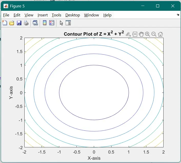
Contour: It is a function/command used for creating a 2d plot using 3d data in form of circular visuals
% Define Data
[X, Y] = meshgrid(-2:0.1:2, -2:0.1:2);
Z = X.^2 + Y.^2;
% Contour Plot
figure;
contour(X, Y, Z);
title('Contour Plot of Z = X^2 + Y^2');
xlabel('X-axis'); ylabel('Y-axis');
OUTPUT:
1.
an input dialogue box is displayed with initial values 0,0
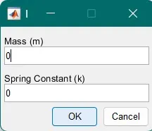
values for both should be given
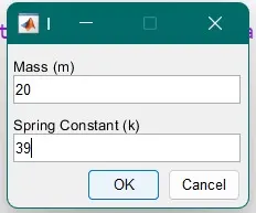
Plots of 45 & 23 are mostly identical. So, we have used different thickness for both in order tee see them.
2.
3.
4.