Project 1 - Data Handling and Interpolation

Project 1 :

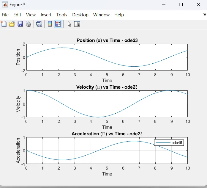
• Solve the simple harmonic oscillator equation [m . dx² / dt² = -k.x ] for a given m (mass) and k (spring constant) values using ‘ode45’ and ‘ode23’ solver in MATLAB.
• Plot x, x_dot (ẋ) & x_dot_dot (ẍ).
• Use the input dialog box to get ‘m’ & ‘k’ values from the user.
• Compare ‘ode45’ and ‘ode23’ plots and explain.

Hint : Refer article on SIMPLE HARMONIC OSCILLATOR and Solving second order differential equation using ODE45

(100 Marks)

ans:

function simpleHarmonicOscillatorComparison()
% Get 'm' and 'k' values from the user using input dialog box
prompt = {'Enter mass (m):', 'Enter spring constant (k):'};
dlgtitle = 'Input Parameters';
dims = [1 35];
defaultValues = {'1.0', '1.0'};
inputValues = inputdlg(prompt, dlgtitle, dims, defaultValues);

m = str2double(inputValues{1});
k = str2double(inputValues{2});

% Time span for the simulation
tspan = [0, 10];

% Initial conditions: x(0) = 0 and x_dot(0) = 1
initialConditions = [0, 1];

% Solve the differential equations using 'ode45' solver
[t_ode45, y_ode45] = ode45(@(t, y) simpleHarmonicOscillatorEquation(t, y, m, k), tspan, initialConditions);

% Solve the differential equations using 'ode23' solver
[t_ode23, y_ode23] = ode23(@(t, y) simpleHarmonicOscillatorEquation(t, y, m, k), tspan, initialConditions);

% Extract x, x_dot, and x_dot_dot from the results
x_ode45 = y_ode45(:, 1);
x_dot_ode45 = y_ode45(:, 2);
x_dot_dot_ode45 = (-k / m) * x_ode45;

x_ode23 = y_ode23(:, 1);
x_dot_ode23 = y_ode23(:, 2);
x_dot_dot_ode23 = (-k / m) * x_ode23;

% Plot the results using 'ode45'
figure;
subplot(3, 1, 1);
plot(t_ode45, x_ode45);
title('Position (x) vs Time - ode45');
xlabel('Time');
ylabel('Position');

subplot(3, 1, 2);
plot(t_ode45, x_dot_ode45);
title('Velocity (ẋ) vs Time - ode45');
xlabel('Time');
ylabel('Velocity');

subplot(3, 1, 3);
plot(t_ode45, x_dot_dot_ode45);
title('Acceleration (ẍ) vs Time - ode45');
xlabel('Time');
ylabel('Acceleration');

% Plot the results using 'ode23'
figure;
subplot(3, 1, 1);
plot(t_ode23, x_ode23);
title('Position (x) vs Time - ode23');
xlabel('Time');
ylabel('Position');

subplot(3, 1, 2);
plot(t_ode23, x_dot_ode23);
title('Velocity (ẋ) vs Time - ode23');
xlabel('Time');
ylabel('Velocity');

subplot(3, 1, 3);
plot(t_ode23, x_dot_dot_ode23);
title('Acceleration (ẍ) vs Time - ode23');
xlabel('Time');
ylabel('Acceleration');

% Legend and grid for both plots
legend('ode45', 'ode23');
grid on;
end

function dydt = simpleHarmonicOscillatorEquation(t, y, m, k)
% y(1) is the position (x)
% y(2) is the velocity (x_dot)

dydt = zeros(2, 1);
dydt(1) = y(2); % x_dot
dydt(2) = (-k / m) * y(1); % x_dot_dot
end

Project 2 :

Write a program to perform the following steps

• load altitude vs temperature data from the tables International Standard Atmosphere (ISA) ((click on the link))
• use the ‘polyfit’ function to determine a regression model: T = f(h) for the above table.
• evaluate the model determined using the ‘polyval’ function
• determine the goodness of fit (goodnessOfFit function)
• Generate comparative plot for the loaded and evaluated data
• store polyval evaluated data into a text file.

(75 Marks)

Project 3 :

Create a function to evaluate the following expression.

y= sin(x²) +cos(x) - 2 sin(x) cos(x)

• Generate the plot and determine all local minima and global maxima values.
• Use the ‘gtext’ command to highlight the local minima and global maxima value in the graph.

Hint: make use of 'fminsearch' & 'max' commands.

(100 Marks)

ans:

The max function will be used to find the global maxima values. The gtext command will allow us to label the local minima and global maxima on the plot.

function evaluate_expression(x_range)x_range = -5:0.1:5;
% Calculate y = sin(x^2) + cos(x) - 2 * sin(x) * cos(x)
y = sin(x_range.^2) + cos(x_range) - 2 * sin(x_range) .* cos(x_range);

% Plot the expression
figure;
plot(x_range, y);
xlabel('x');
ylabel('y');
title('Plot of y = sin(x^2) + cos(x) - 2 * sin(x) * cos(x)');
grid on;

% Find local minima using fminsearch
local_minima_x = [];
local_minima_y = [];
for i = 2:length(x_range)-1
if y(i) < y(i-1) && y(i) < y(i+1)
local_minima_x = [local_minima_x, x_range(i)];
local_minima_y = [local_minima_y, y(i)];
text(x_range(i), y(i), ['Local Minima: (' num2str(x_range(i)) ', ' num2str(y(i)) ')']);
end
end

% Find global maxima using max function
[global_max_y, index] = max(y);
global_max_x = x_range(index);
text(global_max_x, global_max_y, ['Global Maxima: (' num2str(global_max_x) ', ' num2str(global_max_y) ')']);

% Display the plot
disp('Press Enter to close the plot.');
pause;
close(gcf);
end

Project 4 :

Give a brief note on the “contour” command. Illustrate with an example.

Note :

• For example, take simple code and execute in MATLAB.
• Attach the same along with the answer body.

ans:

The contour command in MATLAB is used to create contour plots, also known as level curves. Contour plots are two-dimensional representations of three-dimensional data, where the data points are connected by lines of equal values, forming contours.

The basic syntax for the contour command is:

contour(x,y,z)

• X and Y are matrices representing the coordinates of the data points.
• Z is a matrix representing the data values at each (X, Y) coordinate.

The contour command automatically determines the contour levels based on the data provided and creates a plot with labeled contour lines.

Example:

Let's create a simple example to illustrate the contour command. Consider the following function:

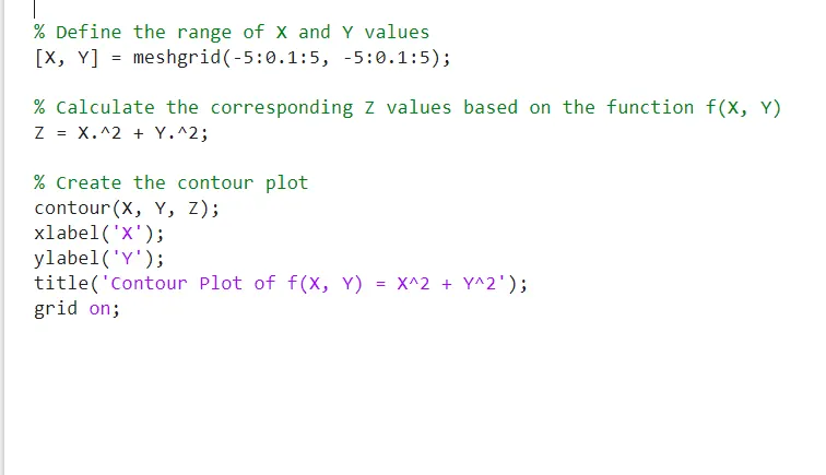
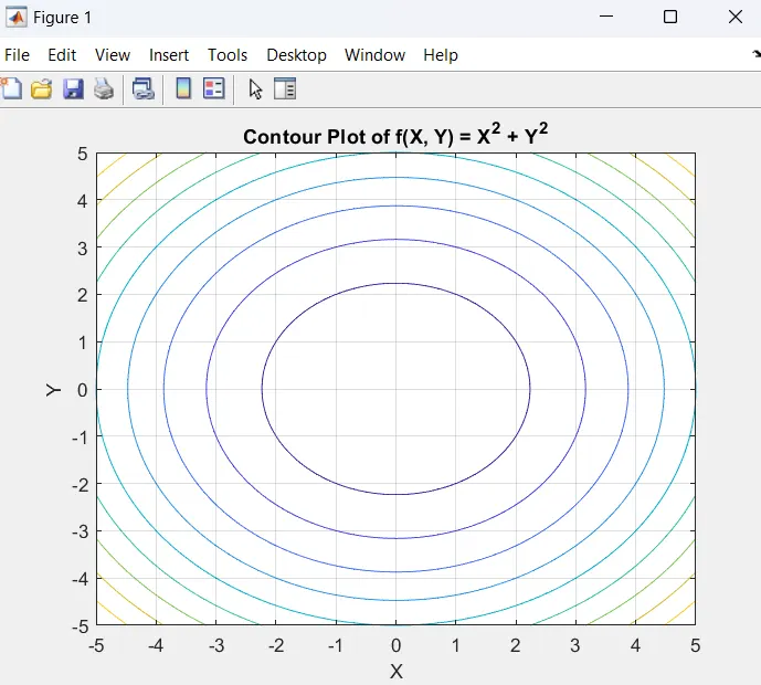
We want to create a contour plot of this function over a specific range of X and Y values.

Contour plots are useful for visualizing 2D data and identifying patterns, regions of interest, or critical points in functions. They are commonly used in scientific, engineering, and data analysis applications.