Challenge

Project 1

GGaneshram Devakumar4 Oct 2024

Aim :

Development of a forward energy-based fuel consumption model of a conventional vehicle.

Objective:

Tabulate the fuel economy numbers (kmpl) for UDDS and HWFET cycle. This forms the baseline numbers for comparing with the future hybrid version.
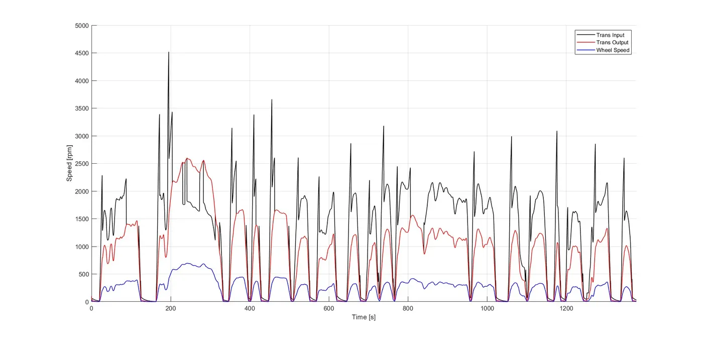
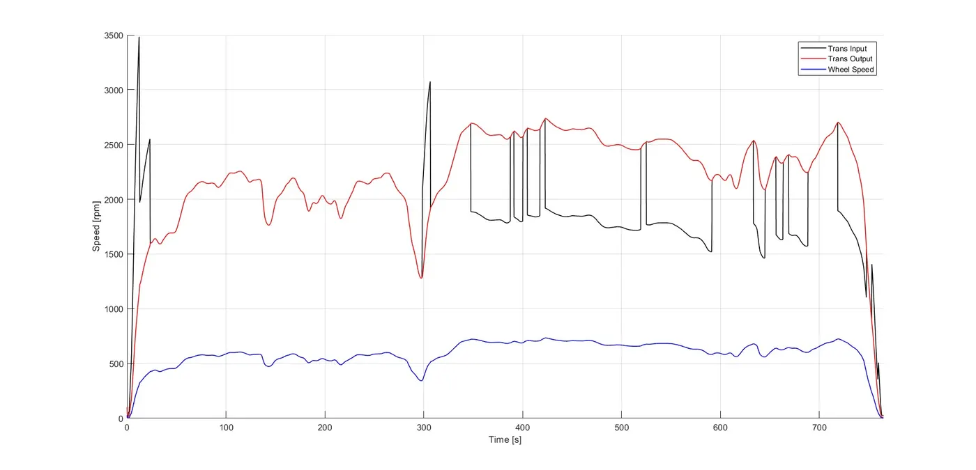
Plot the time trace for engine, transmission input, transmission output and wheel speed on one plot.
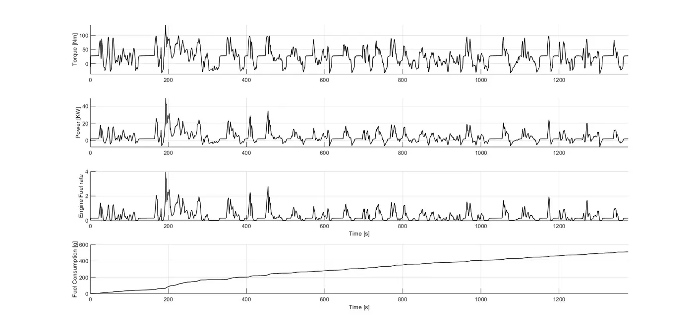
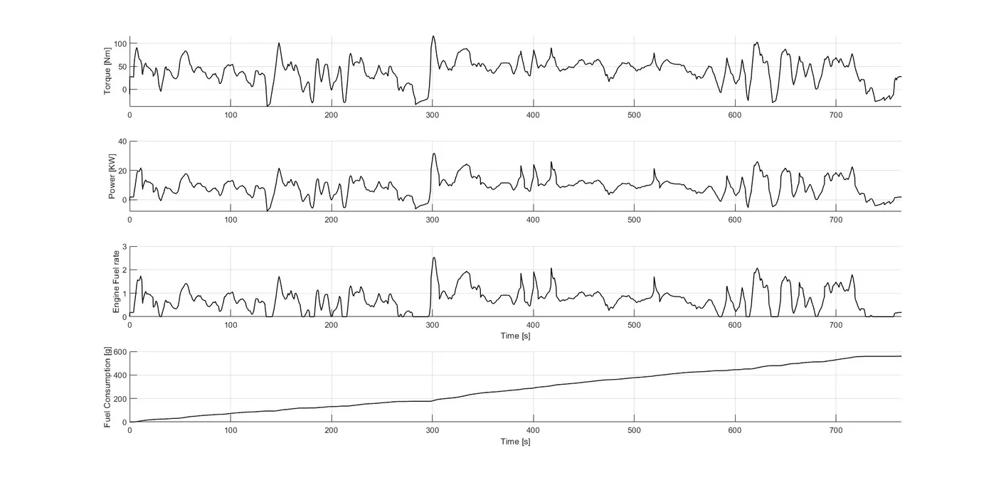
Plot engine torque, engine power, fuel rate and fuel consumption using subplots.
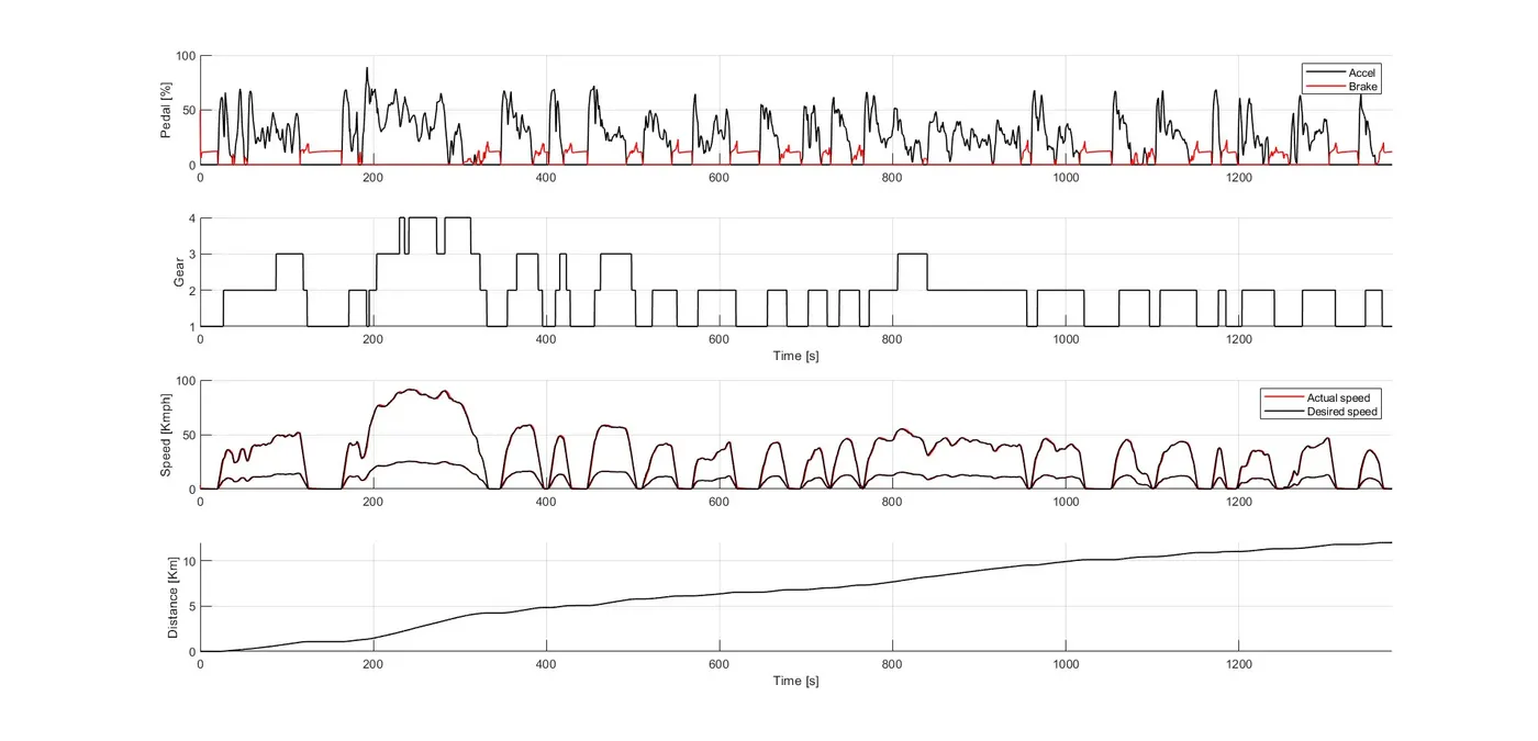
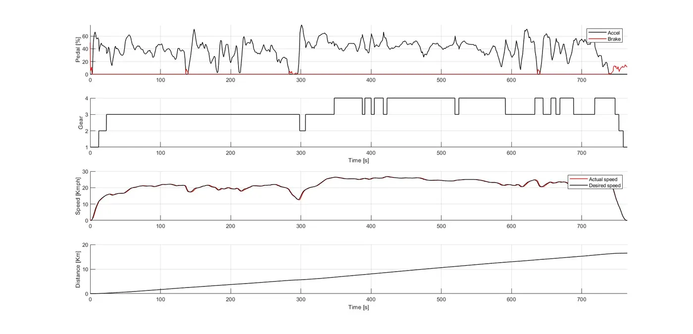
Plot accelerator and brake pedal, gear command, vehicle desired and actual speed, vehicle distance using subplots.
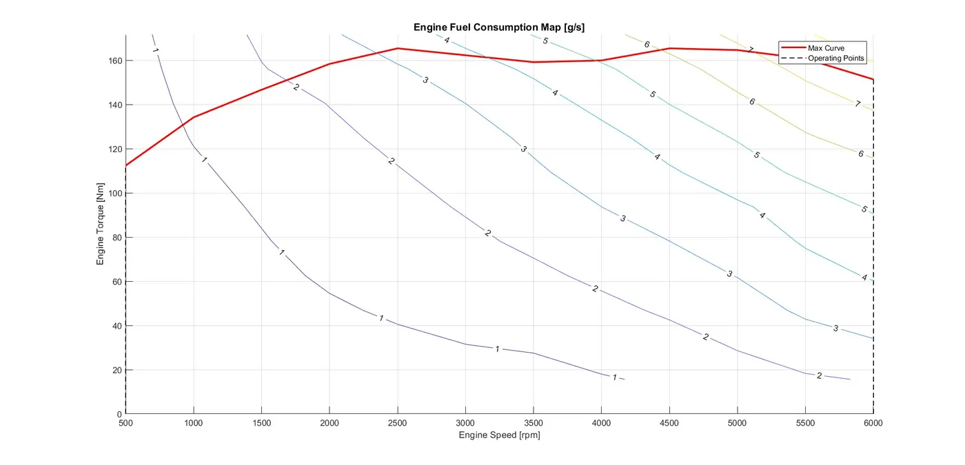
Plot the engine operating points on the engine fuel map.
Write down appropriate brief comments on each of these plots, describing the vehicle behavior throughout the drive cycle.
Generate the plots for both drive cycles.

Introduction –

Conventional fuel vehicles are vehicles that are powered by an internal combustion engine and run on fossil fuels such as petrol or diesel. These vehicles are the most common type in the world and emit significant amounts of carbon dioxide and other pollutants into the atmosphere.

The engine-to-wheel, rear-to-front, and cause-and-effect methods are other names for the forward modelling methodology. Calculation flows from engine to wheel in the same direction as positive power flow.

This method is based on equations for vehicle dynamics, the behavior of individual powertrain parts, and their dynamic interplay.

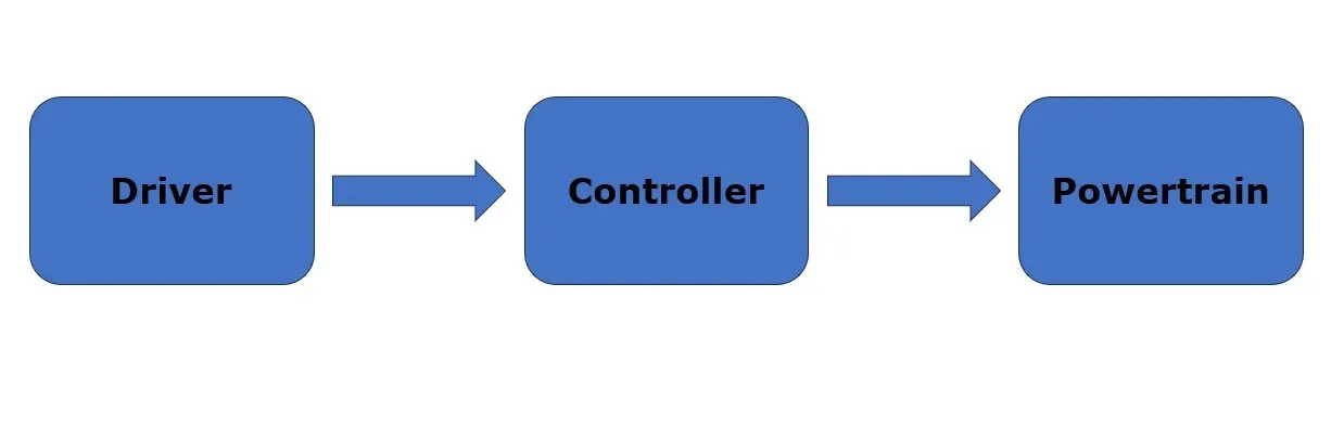
Moreover, a driver controller is necessary to set the calculation start time and operate the vehicle to follow a chosen speed. The controller is set up to simulate how the driver will operate the brakes or the accelerator to match the intended speed, allowing for the study of driver behavior. The controller is utilized as a feedback loop component to calculate the energy necessary to power the vehicle.

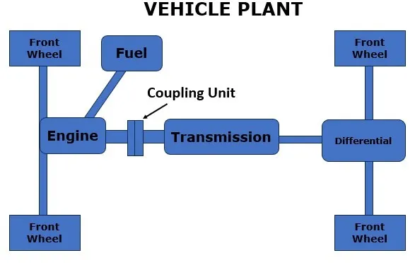
Conventional Powertrain Efficiency:

For a Conventional IC engine vehicle, the wheel power is supplied by the engine through the transmission drivetrain efficiency.

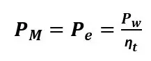
The engine generates power by converting chemical energy stored in the liquid fuel into mechanical energy by the combustion process

This process of energy conversion also has an efficiency vehicle, the wheel power is supplied by the engine through the transmission drivetrain efficiency and the energy input is in the form of fuel consumption.

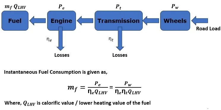
For an IC engine vehicle, even if the power at the wheels is zero, the engine is idling and still consumes some fuel to overcome the engine drag loss and keep it spinning. This is the idling fuel consumption and known as idling losses

Therefore, the formula mentioned previously is applicable only when the wheel power is strictly positive.

When the wheel power is negative, either the engine is disengaged and idling or the engine is engaged and providing some engine braking due to the engine drag losses.

The engine is consuming fuel when it is idling, but even for engine braking, the engine might be consuming some fuel.

In modern engines, fuel is cut-off when decelerating/engine braking to reduce fuel consumption.

Forward energy-based model:

It also known as dynamic simulation. Dynamic models are used for detailed simulations. In this model force/torque/power is the input and the vehicle state variable velocity and acceleration are outputs. The models and simulations are more realistic due to physical casualty hence appropriate for control development. There is feedback loop to meet the desired vehicle state. It is mainly used to simulate a vehicle on a driving cycle to analyze the dynamic behavior of the system helps significantly in control development.

%%%%%%%%%%%%%%%%%%%%%%%%%%%%%%%%%%%%%%%%%%%%%%%%%%%%%%%%%%%%%%%%%%%%%

%% Skill-Lync -> Hybrid Drives Development

% Project 1 - Conventional Vehicle Model

% By - Ganeshram D

% Description:

%% Initialization File

% Initialization file for loading the variables for the Conventional vehicle simulation model

%% Vehicle Parameters

M = 1500; % Vehicle weight [kg]

Cr = 0.015; % Rolling resistance coefficient

Rw = 0.35; % Rolling radius [m]

Cd = 0.33; % Drag coefficient

Af = 2; % Frontal area [m2]

rhoa = 1.225; % Air density [kg/m3]

Vwind = 0; % Wind velocity [kmph]

g = 9.81; % Gravitational acceleration [m/s2]

theta = 0; % Slope [deg]

myu_road_tire = 1; % Coefficient of friction between tire - road interface

%% Powertrain Parameters

FDR = 3.73; % Final Drive Ratio / Diff Ratio

DiffEff = 0.99; % Differential efficiency (assumed independent of operating conditions)

NumGear = 4; % Number of gears in transmission

TransGear = [1:NumGear]; % Transmission Gears

TransRatio = [3.06, 1.62, 1, 0.7]; % Corresponding Transmission ratios

TransEff = 0.90; % Transmission efficiency (assumed independent of operating conditions)

TC_SR = [0, .5, .6, .7, .8, .87, .92, .94, .96, .97, 1]; % Torque Converter Speed Ratio (Matlab default) -> TurbSpd/PumpSpd

TC_TR = [2.232, 1.5462, 1.4058, 1.2746, 1.1528, 1.0732, 1.0192, 1, 1, 1, 1]; % Torque Converter Torque Ratio (Matlab default) -> TurbTrq/PumpTrq

TC_Cf = 1e-4 * [.72558, .66322, .63463, .59042, .51331, .4144, .29287, .22444, .12186, .04386, 0]; % Torque Converter Capacity Factor (Matlab default) -> PumpTrq/PumpSpd^2 [Nm/rpm^2]

load Vehicle_Data/Engine_data_1_9L_Saturn_95kW

load Vehicle_Data/Trans_Shift_map

%% Driver Parameters

Kp = 10; % P gain for driver PI model

Ki = 1; % I gain for driver PI model

Drive_Cycle_Select = 1; % Drive cycle selection

% Drive cycle values in m/s

if Drive_Cycle_Select == 1

load DriveCycles/UDDS;

elseif Drive_Cycle_Select == 2

load DriveCycles/HWFET;

elseif Drive_Cycle_Select == 3

load DriveCycles/FTP;

elseif Drive_Cycle_Select == 4

load DriveCycles/US06;

elseif Drive_Cycle_Select == 5

load DriveCycles/NEDC;

elseif Drive_Cycle_Select == 6

load DriveCycles/WLTP;

end

time_end = cyc_time(end);

vel_end = cyc_vel(end);

Simulink model of conventional vehicle: In this project, a typical midsize car with a 1.9L engine and a 4-speed automatic transmission is considered.

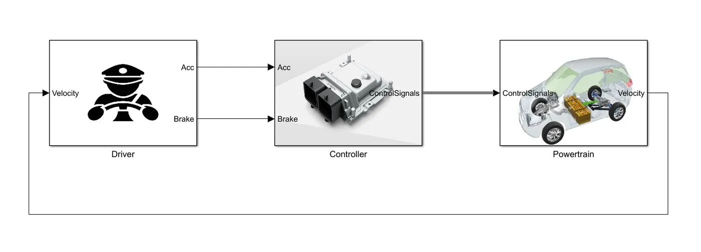
The Simulink model for the convection vehicle model having 3 main subsystem for the driver model, control model and powertrain block.

The actual vehicle speed is given as feedback to the driver block, and the driver block gives the controller block the required acceleration, torque, brake and power output, while the controller block provides control signals for engine torque, gear shifting and brake torque to the Powertrain model.

Driver Model:

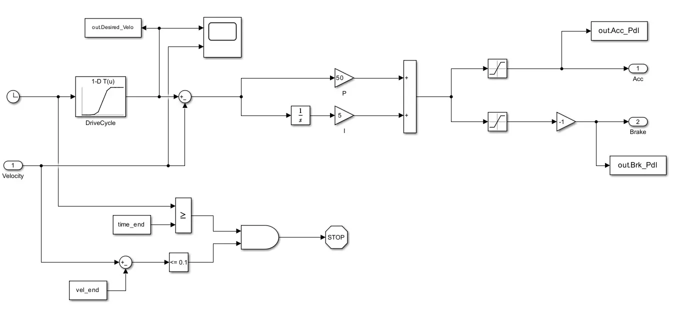
Driver Model is a basic PI controller that generates accelerator and brake pedal outputs to match the desired and actual vehicle speeds. The Proportional and integrator controls the error between desired output and actual speed through feedback controls

Controller Model:

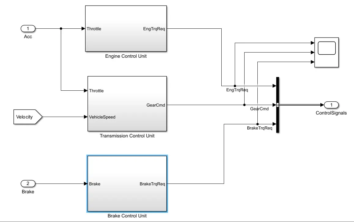
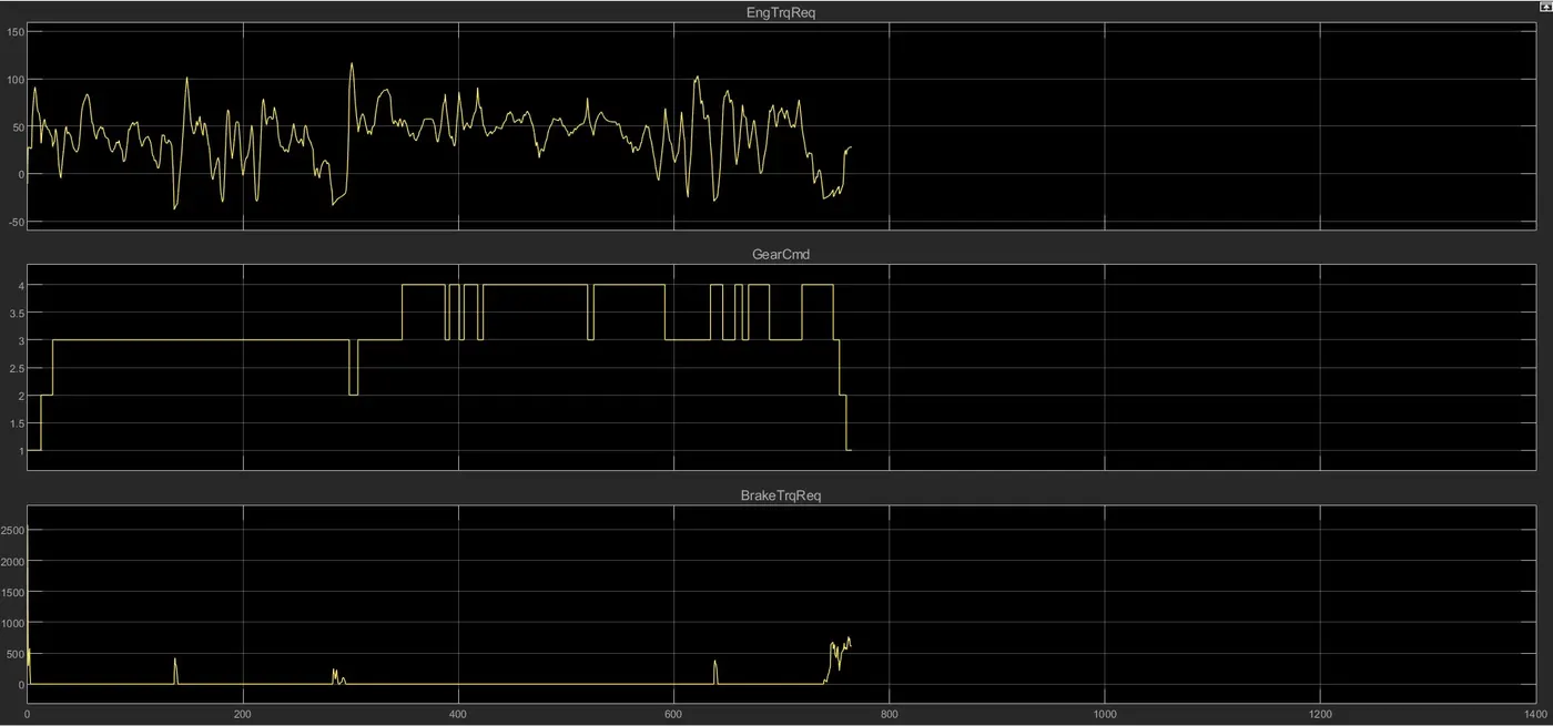
The Controller subsystem having engine, transmission and brake control unit which is act a heart of the conventional vehicle. Based on the driver input appropriate signal is transmitted to the all the sub system to deliver the desired engine torque, desired speed, desired brake torque. these signals are transmitted to powertrain to deliver driver desired outputs.

Scope Results of Controller:

Engine Control Unit &

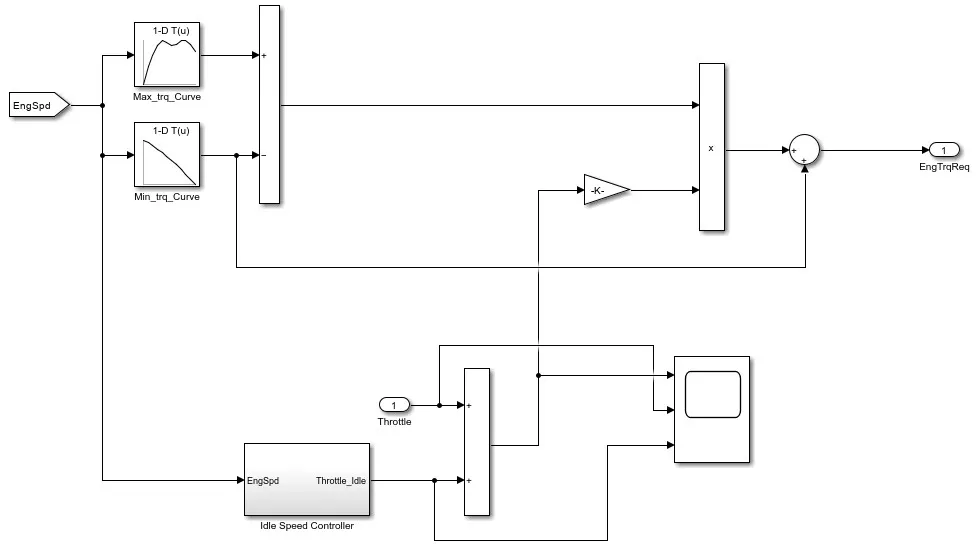
Engine Control Unit Compare engine speed with the maximum torque and minimum torque curves of the lookup table and give the required torque command to the engine block.

Idle Speed Controller:

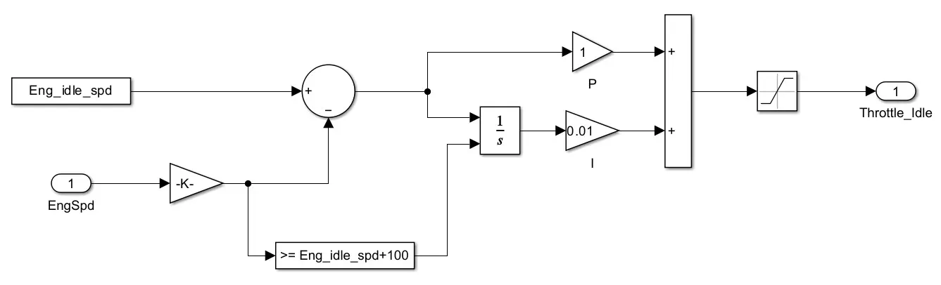
The throttle input is combined with the idle speed throttle and gains with the torque output from the lookup table to estimate the torque input required for the engine.

Transmission Control Block:

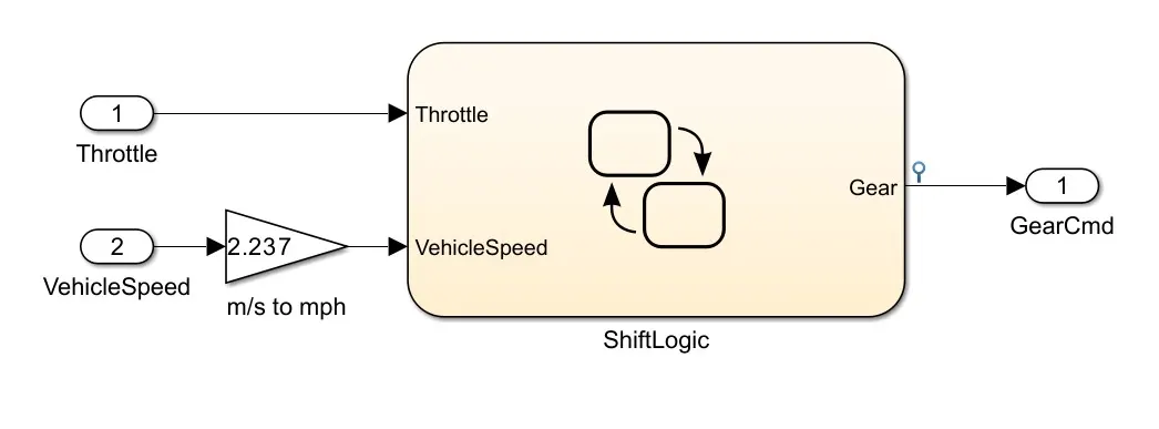
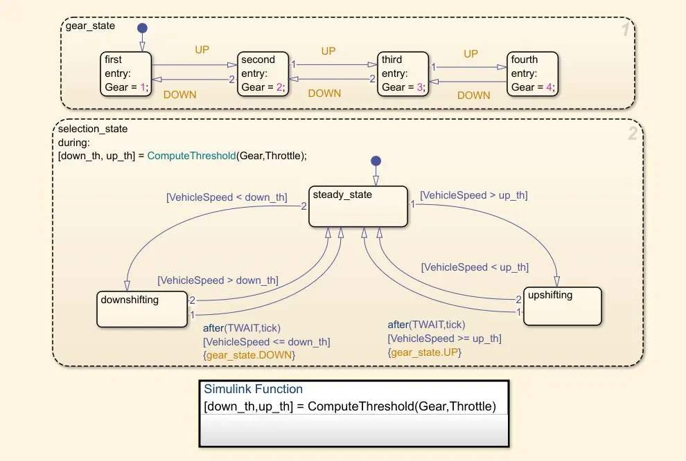
The transmission control block controls the gear shifting using the study flow Variable chart. The Gear shifting is Controlled according to the vehicle speed and throttle input. The gear command is passed to the Transmission block to select the desired gear ratio.

Brake Control Unit:

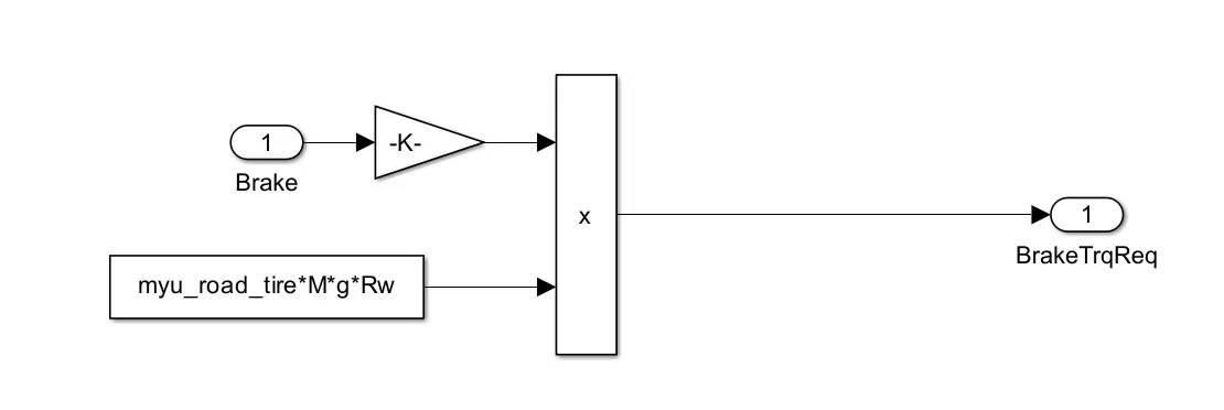
Brake Control unit Produce required brake torque according to the brake pedal input and passes the brake torque in to the wheel block in the transmission model.

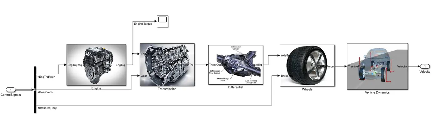
Powertrain Model:

The powertrain model includes all the components that convert the power of the engine into vehicle motion. This includes Engine, Transmission, Differential, Wheels and the vehicle body dynamics subsystems.

Engine Model:

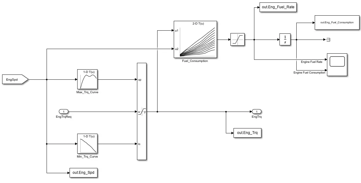
Based on the Engine speed The required torque from the controller is saturated between Max torque curve and min torque curve and passes the Engine torque to the Transmission block

The 2D lookup table is used to calculate the fuel flow rate based on engine speed and engine torque. The fuel flow rate is then integrated to find the fuel consumption.

Estimated fuel flow rate, fuel consumption, engine torque and engine speed are passed to the MATLAB workspace using the to-workspace block.

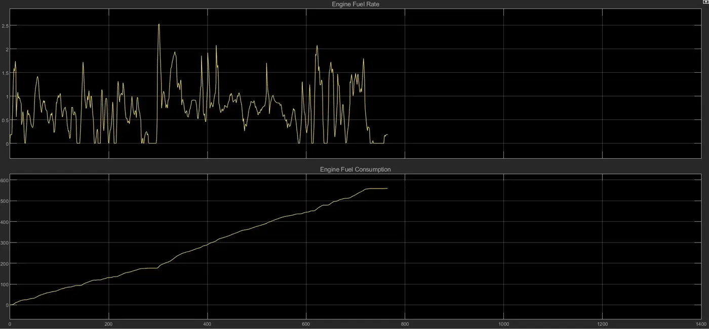
Scope Results of Engine:

Transmission Model:

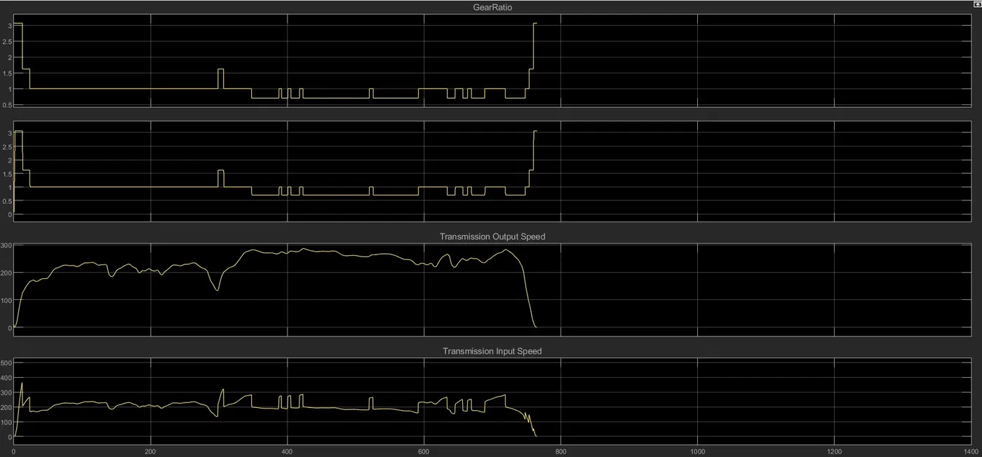
The engine block is connected to the automatic transmission via a torque converter. The output of the transmission is connected to the differential.

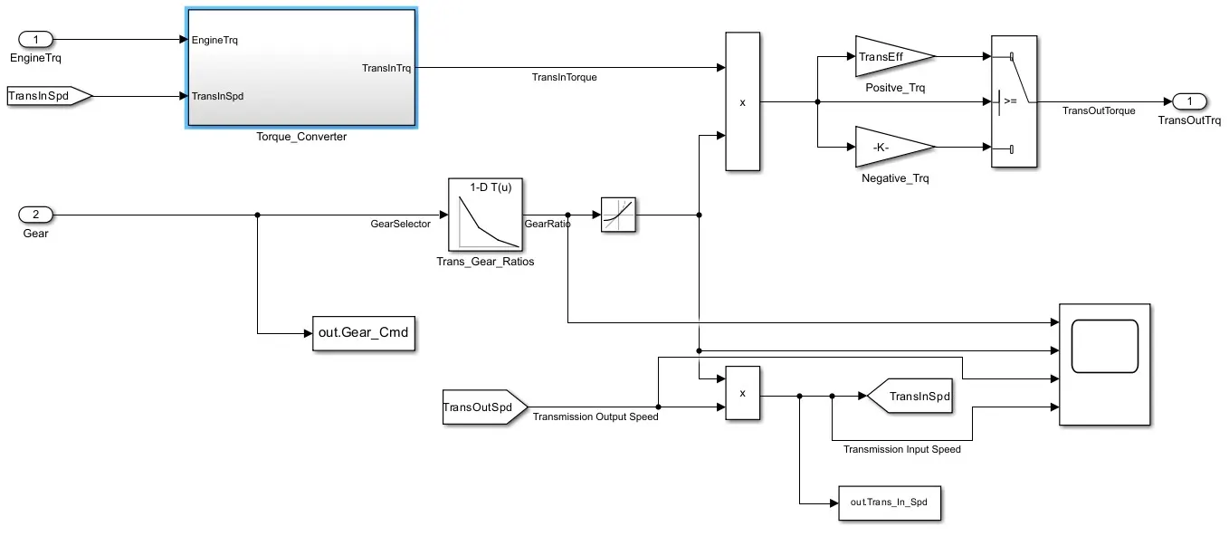
Scope Results of Transmission:

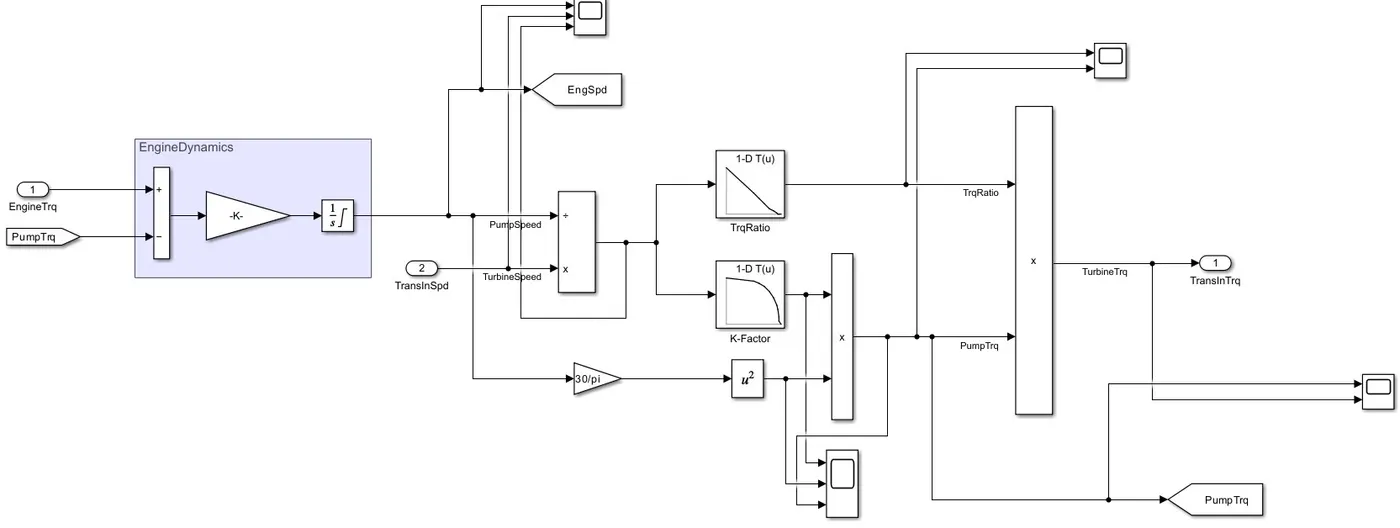
Torque Converter:

The gear selection from the transmission control unit is multiplied by the engine torque in this block, and the efficiency and engine dynamics of the torque converter are applied in this model.

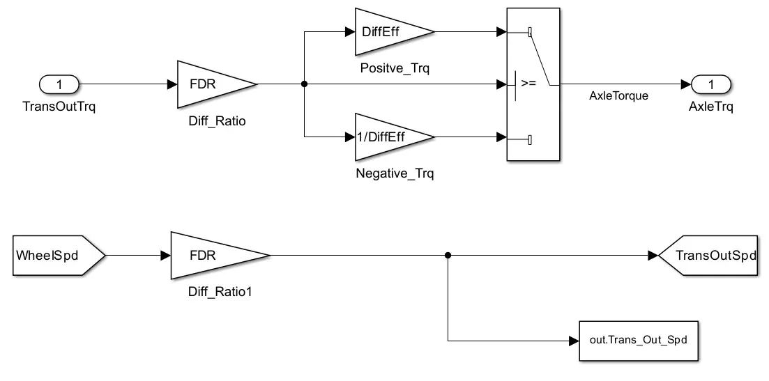
Differential Model:

The transmission output torque is multiplied by the differential ratio and differential efficiency in this block and the torque is transmitted to the wheel as the axle torque.

Wheel Model:

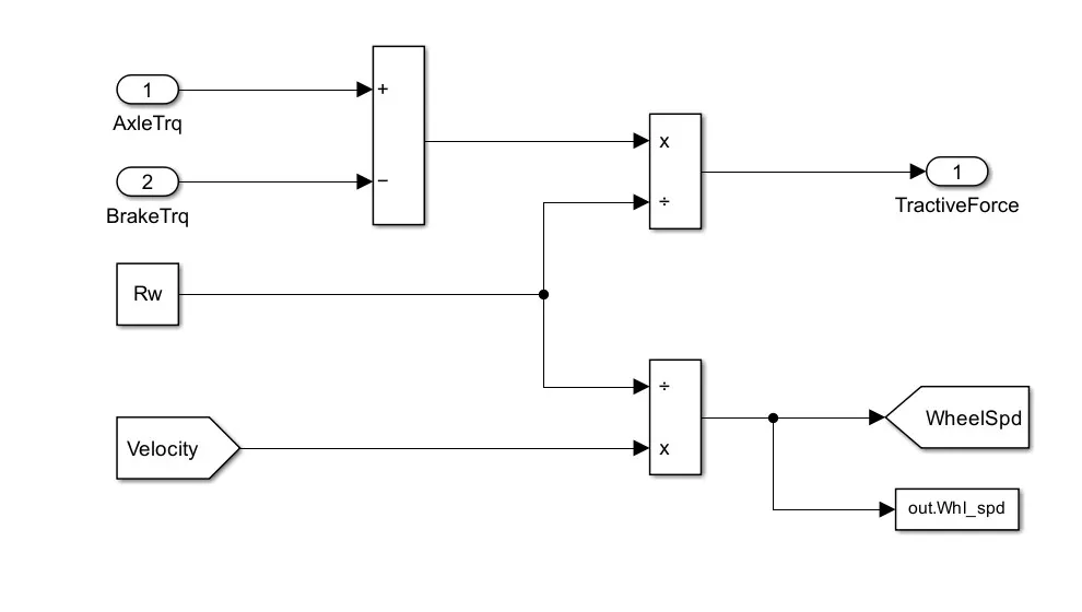
The brake torque from the control model is subtracted from the Axle torque and divides from the rolling radius to determine the Tractive force. The Wheel speed is calculated from the vehicle velocity.

Vehicle Dynamics Model:

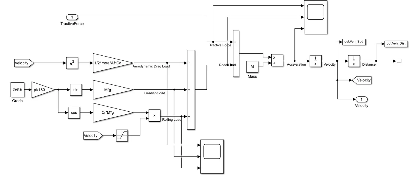
The longitudinal dynamics of the vehicle along with the road load is represented in the ‘Vehicle Dynamics’ block

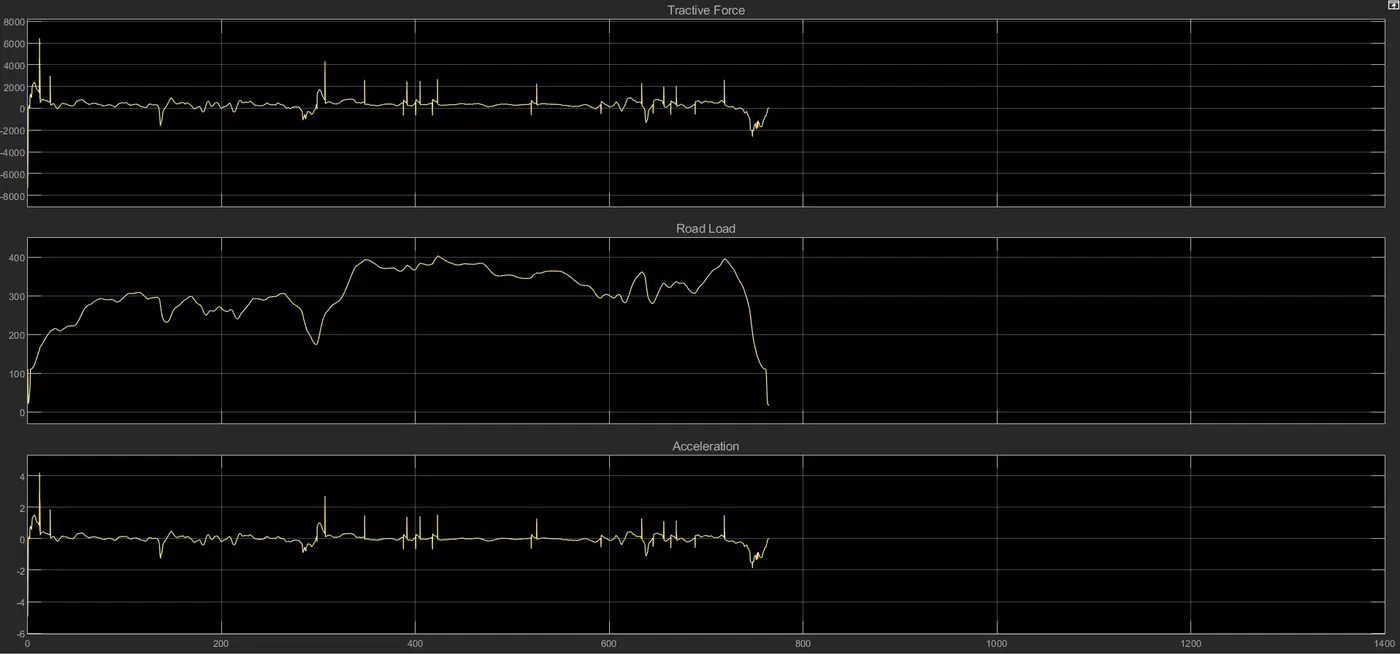
Scope Results of Vehicle Dynamics:

Listing forces different applicable as per the scenario

Tractive effort and resistance are the two main forces that oppose one another and determine the performance of roadway vehicles. Tractive effort is the force exerted against the roadway surface to allow a vehicle to move forward. Resistance encompasses all forces that push back and impede motion. Both of these are in units of force.

Rolling Resistance

Rolling resistance is caused by the interaction of tires with the roadway surface. Three main causes exist that create this resistance. The first is the rigidity of the tire and the roadway surface. The second is tire pressure and temperature. The third is vehicular operating speed.

Aerodynamic Resistance

Aerodynamic resistance is a force that is produced by turbulent air flow around the vehicle body. This turbulence is dependent on the shape of the vehicle, as well as the friction of air passing over the vehicle's surface. A small portion of this resistance comes from air flow through vehicle components, such as interior ventilation.

Grade Resistance

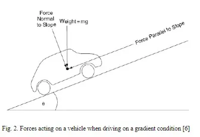
Grade resistance is the simplest form of resistance. It is the gravitational force acting on the vehicle. This force may not be exactly perpendicular to the roadway surface, especially in situations when a grade is present. Angle created between horizontal and the slope is θ. Several industrial vehicle manufacturers call the ability of the vehicle to run on a slope as Gradeability. Unit for gradeability is percent. Gradeability is calculated by multiplying tan θ with 100%.

Acceleration –

Inertia is force that inhibits the vehicle to reach a certain speed in a certain time. It is impossible for vehicle to achieve a certain speed from its idle position without acceleration. Therefore, to get to certain speed, the vehicle should be able to perform acceleration.

Power required at wheels is given by:

The power required at the wheels of a vehicle can be calculated using the formula P = Fv, where P is power, F is force, and v is velocity.

Modified MATLAB Script for Post Processing:

The given MATLAB script is modified to analyze data and generate plots. Here we rename the variables loaded from the model, do some basic post-process calculations and generate results and plots.

%%%%%%%%%%%%%%%%%%%%%%%%%%%%%%%%%%%%%%%%%%%%%%%%%%%%%%%%%%%%%%%%%%%%%

%% Skill-Lync -> Hybrid Drives Development

% Project 1 - Conventional Vehicle Model

% By - Ganeshram D

% Description:

% The following file is to used with the Initialization file and Simulink

% results for post-processing of the data.

% The file is incomplete, has some examples of how the data is imported

% into a readable format, data analysis and plotting examples.

% Based on the project task, use commands in a similar format as given

% below, to analyse the data and generate required plots.

% You can change variable names if desired

%% Post-Processing File

% File for post-processing the Conventional vehicle simulation model data

%% Renaming variables

Time = out.tout;

Acc_Pdl = out.Acc_Pdl; % Accelerator pedal [%]

Brk_Pdl = out.Brk_Pdl; % Brake pedal [%]

Gear_Cmd = out.Gear_Cmd; % Transmission gear

Trans_In_Spd = out.Trans_In_Spd*30/pi; % Transmission input speed [rpm]

Trans_Out_Spd = out.Trans_Out_Spd*30/pi;% Transmission output speed [rpm]

Eng_Trq = out.Eng_Trq; % Engine brake torque [Nm]

Eng_Spd = out.Eng_Spd*30/pi; % Engine speed [rpm]

Eng_Fuel_rate = out.Eng_Fuel_Rate; % Engine Fuel Rate [g\kW]

Eng_Fuel_Consump = out.Eng_Fuel_Consumption; % Engine fuel consumption [g]

Veh_Dist = out.Veh_Dist/1000; % Distance traveled by vehicle [km]

Veh_Spd = out.Veh_Spd; % Vehicle speed [m/s]

Whl_Spd = out.Whl_spd*30/pi; % Wheel speed [rpm]

Desired_spd = out.Desired_Velo; % Desired Speed [m/s]

%% Data Analysis

Eng_Pwr = Eng_Spd*pi/30.*Eng_Trq/1000; % Engine brake power [kW]

rho_petrol = 0.7197; % Density of petrol [kg/L]

kmpl = Veh_Dist(end)/(Eng_Fuel_Consump(end)/1000/rho_petrol); % Fuel economy [kmpl]

%% Plotting vehicle characteristics time trace

% Plotting transmission input, transmission output and wheel speed

figure(1)

hold on

grid on

plot(Time, Trans_In_Spd, 'linewidth', 1, 'Color', 'black');

plot(Time, Trans_Out_Spd, 'linewidth', 1, 'Color', 'red');

plot(Time, Whl_Spd, 'linewidth', 1, 'Color', 'blue');

xlabel('Time [s]')

ylabel('Speed [rpm]')

xlim([0, Time(end)]);

legend('Trans Input','Trans Output','Wheel Speed');

% Plotting engine torque, engine power, fuel rate and fuel consumption

figure(2)

subplot(4,1,1)

hold on

grid on

plot(Time, Eng_Trq, 'linewidth', 1, 'Color', 'black');

ylabel('Torque [Nm]')

xlim([0, Time(end)]);

subplot(4,1,2)

hold on

grid on

plot(Time, Eng_Pwr, 'linewidth', 1, 'Color', 'black');

ylabel('Power [KW]')

xlim([0, Time(end)]);

subplot(4,1,3)

hold on

grid on

plot(Time, Eng_Fuel_rate, 'linewidth', 1, 'Color', 'black');

xlim([0, Time(end)]);

xlabel('Time [s]');

ylabel('Engine Fuel rate');

subplot(4,1,4)

hold on

grid on

plot(Time, Eng_Fuel_Consump, 'linewidth', 1, 'Color', 'black');

xlim([0, Time(end)]);

xlabel('Time [s]');

ylabel('Fuel Consumption [g]');

%Plotting accelerator and brake pedal gear command, vehicle desired and actual speed, vehicle distance

figure(3)

subplot(4,1,1)

hold on

grid on

plot(Time, Acc_Pdl, 'linewidth', 1, 'Color', 'black');

plot(Time, Brk_Pdl, 'linewidth', 1, 'Color', 'red');

ylabel('Pedal [%]')

xlim([0, Time(end)]);

legend('Accel','Brake');

subplot(4,1,2)

hold on

grid on

plot(Time, Gear_Cmd, 'linewidth', 1, 'Color', 'black');

xlim([0, Time(end)]);

xlabel('Time [s]');

ylabel('Gear');

subplot(4,1,3)

hold on

grid on

plot(Time, Veh_Spd, 'linewidth', 1, 'Color', 'red');

plot(Time, Desired_spd, 'linewidth', 1, 'Color', 'black');

ylabel('Speed [Kmph]')

xlim([0, Time(end)]);

legend('Actual speed','Desired speed');

subplot(4,1,4)

hold on

grid on

plot(Time, Veh_Dist, 'linewidth', 1, 'Color', 'black');

xlim([0, Time(end)]);

xlabel('Time [s]');

ylabel('Distance [Km]');

%% Plotting Drive Cycle

figure(4)

hold on

grid on

plot(cyc_time, cyc_vel, 'linewidth', 1, 'Color', 'black');

xlabel('Time [s]')

ylabel('Velocity [Mph]')

title('Drive Cycle')

% Tabulation of Test Results

Avg_speed = sum(Veh_Spd)/length(Veh_Spd);

Max_Speed = maxk(Veh_Spd,1);

table(Avg_speed,Max_Speed,kmpl,'VariableNames',{'Average Speed [m/s]','Maximum Speed [m/s]','Fuel Economy [kmpl]'})

%% Plotting engine operating points on engine fuel map

figure('Name','Engine Operating Points');

hold on

grid on

title('Engine Operating Points','fontsize',12);

p1=plot(Eng_map_spd*30/pi,Eng_max_trq,'linewidth',2,'color','r');

p2=line([Eng_map_spd(end)*30/pi Eng_map_spd(end)*30/pi],[0 Eng_max_trq(end)]);

set(p2,'linewidth',1,'linestyle','--','color','k');

p3=line([Eng_map_spd(1)*30/pi Eng_map_spd(1)*30/pi],[0 Eng_max_trq(1)]);

set(p3,'linewidth',1,'linestyle','--','color','k');

[c,h] = contour(Eng_map_spd'*30/pi,Eng_map_trq,Eng_fuel_map');

clabel(c,h);

xlabel('Engine Speed [rpm]');

ylabel('Engine Torque [Nm]');

title('Engine Fuel Consumption Map [g/s]');

legend({'Max Curve','Operating Points'});

axis([Eng_map_spd(1)*30/pi Eng_map_spd(end)*30/pi 0 Eng_map_trq(end)]);

Output Results:

#1 Tabulate the fuel economy numbers (kmpl) for UDDS and HWFET cycle.

UDDS Drive Cycle -

HWFET Drive Cycle -

#1 Comments -

The fuel economy of the typical midsize car having a 1.9L engine and a 4-speed automatic transmission is higher in the highway driving condition compare to urban driving condition where frequent stoppage of vehicle can experience.

#2 Plot the time trace for engine, transmission input, transmission output and wheel speed

UDDS Drive Cycle -

HWFET Drive Cycle -

#2 Comments -

In UDDS drive cycle, Due to the frequent stoppage and idle loss, the input speed is facilitated by the torque converter and the transmission input speed fluctuates according to the engine torque required to achieve the drive cycle. But in Highway drive cycle, the speed flotation is comparatively less (almost nil) and no idle losses. Wheel speed and transmission output speed vary according to gear and differential ratio.

#3 Plot engine torque, engine power, fuel rate and fuel consumption:

UDDS Drive Cycle -

HWFET Drive Cycle -

#3 Comments -

In UDDS drive cycle, Due to the frequent stoppage and idle loss, torque, Power requirements are less compared to the HWFET drive cycle which has high torque and power requirements

#4 Plot accelerator and brake pedal, gear command, vehicle desired and actual speed, vehicle distance

UDDS Drive Cycle -

HWFET Drive Cycle -

#4 Comments –

In UDDS Drive cycle, Brake requirements are higher, less accelerator pedals and gear shifts often occur because this drive cycle is running with fluctuating speed, but in HWFET drive cycle Brake requirements are lower, more accelerator pedals are applied on the highway drive cycle, and gear shifts often occur because the drive cycle is smoother

#5 Plot the engine operating points on the engine fuel map

UDDS Drive Cycle -

HWFET Drive Cycle -

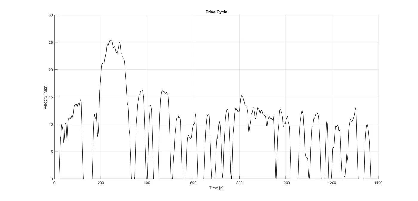
#6 Generate the plots for both drive cycles

UDDS Drive Cycle -

HWFET Drive Cycle -

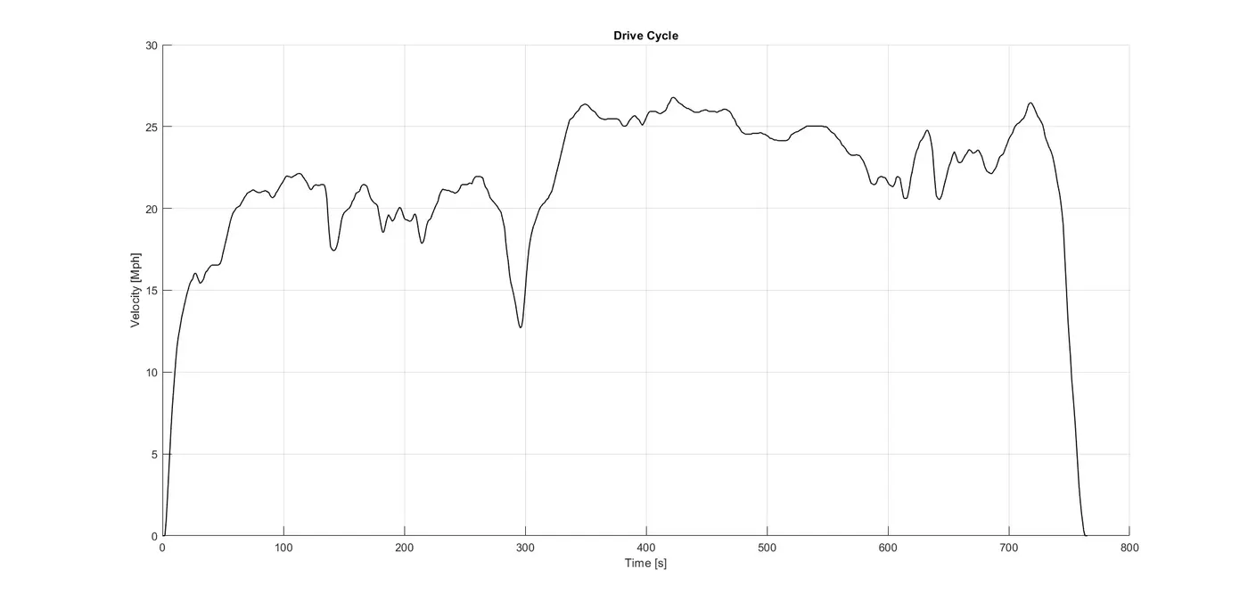
#6 Comments -

In UDDS drive cycle, velocity/speed of the vehicle is fluctuating over the time due to running in urban roads where the frequent stoppage and idle losses are more compare to High drive cycle.

In HWFET drive cycle, velocity/speed of the vehicle is comparatively less (almost nil) and no idle losses. Hence the distance covered by the high way driven condition vehicle is more compare to urban driven condition driven

Conclusion:

The forward energy-based fuel consumption model of a conventional vehicle has been successfully Simulated using MATLAB and Simulink.
Analyses and understands vehicle operating points based on engine speed, torque, transmission speed, pedal positions, gear, and distance travelled.
Post process calculations were performed and the required graphs were successfully plotted.
Successfully calculated vehicle fuel efficiency numbers (kmpl) for the given urban drive cycle (UDDS) and highway cycle (HWFET).

Project 1

Ship work like this
in your own course.

Talk to a career counsellor

Ship work like thisin your own course.

Talk to a career counsellor

Ship work like this
in your own course.