Project 1
Objective:-> To solve the 2D steady and unsteady (Transient) heat conduction equations by using the point iterative techniques.
Following iterative technique can be used.
- Jacobi
- Gauss-seidel
- Successive over-relaxation
Given data:-
Top Boundary = 600 K
Bottom Boundary = 900 K
Left Boundary = 400 K
Right Boundary = 800 K
Let us consider a square plate with boundary length of 1m. The number of grid points on X-axis & Y-axis 10.
α=α= Thermal diffusivity = 1.4 (m^2/s)
Convergence criteria Tolerance = 0.0001
We know heat always transfer from high temperature point to low temperature point.
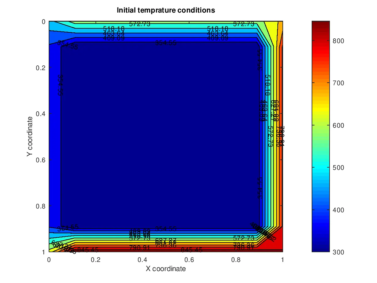
1. Steady-state condition:- Under this condition temperature within the system remains unchanged with respect to change in time.
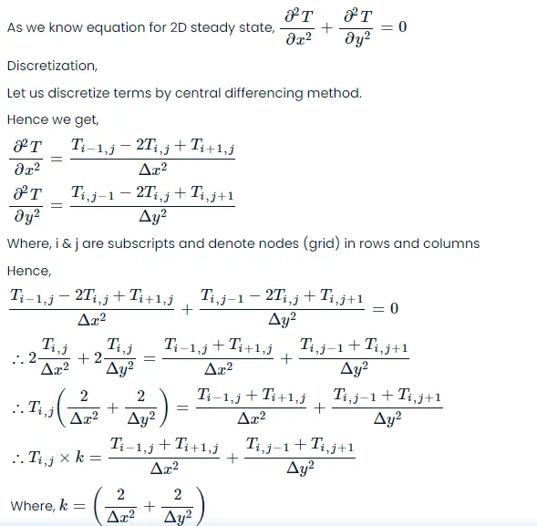
MATLAB Code for Steady state condition:-
Let us create code by considering above condition and equation.
clear all
close all
clc

L=1; %Length of square domain in meter
nx=ny=10; %Number of nodes (gridpoints)
%Mesh creation
x=linspace(0,L,nx);
dx=L/(nx-1); %Meshing in X direction
y=linspace(0,L,ny);
dy=L/(ny-1); %Meshing in Y direction

%2D matrix creation
[X,Y] = meshgrid(x,y);

%Initialization
T=300*ones(nx,ny);
T(:,1)=400; %Temperature at left wall
T(:,nx)=800; %Temperature at right wall
T(1,:)=600; %Temperature at top wall
T(ny,:)=900; %Temperature at bottom wall
T(1,1)=(400+600)/2; %Temperature at top left corner
T(nx,1)=(400+900)/2; %Temperature at bottom left corner
T(1,ny)=(600+800)/2; %Temperature at top right corner
T(nx,ny)=(800+900)/2; %Temperature at bottom right corner

Told=T;
k=(2/(dx)^2 + 2/(dy)^2);

tol=1e-4; %Convergence criteria

%Input method number
method= input('Enter method number 1.Jacobi 2.GS 3.SOR: ')

tic;
%Jacobian method
if method==1
  itr_jaco = 1;
  error=9e9; %error reinitialization
  %Convergence loop
  while error > tol
    %space loop
    for i=2:nx-1
      for j=2:ny-1
        T(i,j)=((Told(i-1,j)+Told(i+1,j))/(dx)^2 + (Told(i,j-1)+Told(i,j+1))/(dy)^2)/k;
      endfor
    endfor

  error_n=abs(max(T-Told));
  error = max(error_n);
  Told=T; %Reinitialization of temprature
  itr_jaco = itr_jaco + 1;

  %Plotting
  figure(1)
  colormap(jet);
  [c,h] = contourf(x,y,T,'showtext','on');
  set(gca,'YDIR','reverse');
  colorbar;
  xlabel('X coordinate');
  ylabel('Y coordinate');
  title(['Jacobian iteration value = ',num2str(itr_jaco)]);
  pause(0.01);
  %Ellapsed time = 542.28
  endwhile

%GS
elseif method==2
  itr_gs = 1;
  error=9e9; %error reinitialization
  %Convergence loop
  while error > tol
    %space loop
    for i=2:nx-1
      for j=2:ny-1
        T(i,j)=((T(i-1,j)+Told(i+1,j))/(dx)^2 + (T(i,j-1)+Told(i,j+1))/(dy)^2)/k;
      endfor
    endfor
    error_n=abs(max(T-Told));
    error = max(error_n);
    Told=T; %Reinitialization temprature
    itr_gs = itr_gs + 1;

    %plotting
    figure(2)
    colormap(jet);
    [c,h] = contourf(x,y,T,'showtext','on');
    set(gca,'YDIR','reverse');
    colorbar;
    xlabel('X coordinate');
    ylabel('Y coordinate');
    title(['GS iteration value = ',num2str(itr_gs)]);
    pause(0.01);
    %Ellapsed time = 382.46
  endwhile

%SOR
elseif method==3
  itr_sor = 1;
  error=9e9; %error reinitialization
  %for w=0.8, No. of iterations = 164
  %for w=0.9, No. of iterations = 136
  %for w=1.0, No. of iterations = 112
  %for w=1.1, No. of iterations = 93
  %for w=1.2, No. of iterations = 76
  %for w=1.3, No. of iterations = 60
  %for w=1.4, No. of iterations = 46
  %for w=1.5, No. of iterations = 28
  %for w=1.6, No. of iterations = 35
  %for w=1.55, No. of iterations = 35
  w=1.51; %over relaxation

  %convergence loop
  while error > tol
    %space loop
    for i=2:nx-1
      for j=2:ny-1
        T(i,j)=(1-w)*Told(i,j) + (w*((T(i-1,j)+Told(i+1,j))/(dx)^2 + (T(i,j-1)+Told(i,j+1))/(dy)^2)/k);
      endfor
    endfor
    error_n=abs(max(T-Told));
    error = max(error_n);
    Told=T; %Reinitialization temperature
    itr_sor = itr_sor + 1;

    %plotting
    figure(3)
    colormap(jet);
    [c,h] = contourf(x,y,T,'showtext','on');
    set(gca,'YDIR','reverse');
    colorbar;
    xlabel('X coordinate');
    ylabel('Y coordinate');
    title(['SOR iteration value = ',num2str(itr_sor)]);
    pause(0.01);
    %Ellapsed time = 102.00
  endwhile
end
Ellapsed_time=toc
Above code consist of all 3 iterative solvers. When user enter 1 then code of Jacobian iterative solver starts running and display output on graph. Similarly, when user enter 2 then code for Gauss-Seidel iterative solver starts running and when user enter 3 then SOR code will run.
I. Jacobian solver
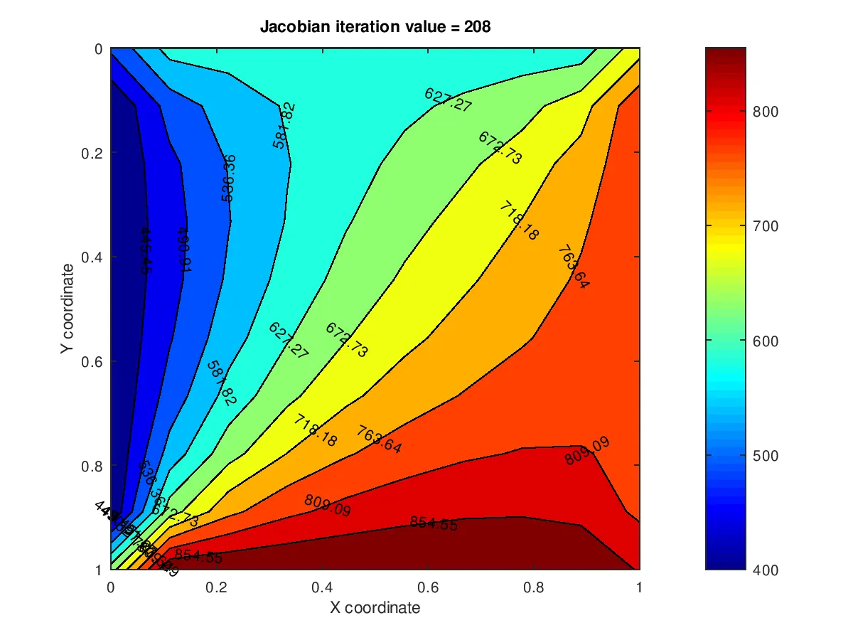
Above plot shows temperature profile by Jacobian solver. For solution convergence Jacobian solver required 208 iterations.
II. Gauss- Seidel solver
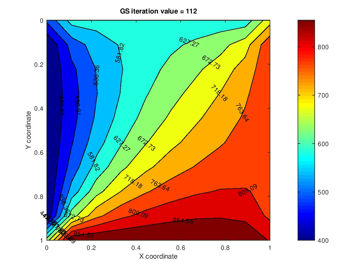
Above plot shows temperature profile by GS solver. For solution convergence this solver required 112 iterations.
III. Successive over relaxation
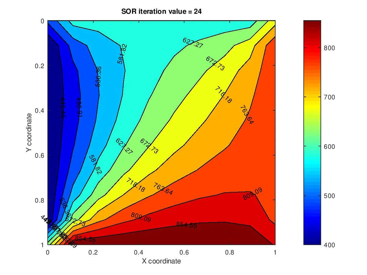
Above plot shows temperature profile by SOR solver. For solution convergence this solver required 24 iterations only. We get least number of iterations for ω=1.51ω=1.51.
2. Transient condition:- For transient heat transfer conditions the temperature within system varies with respect to time.
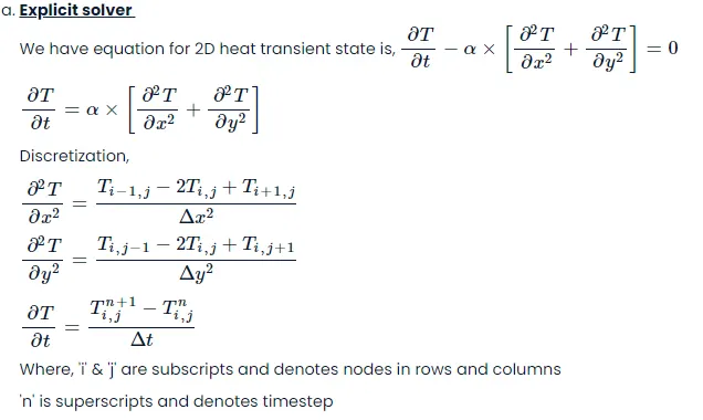
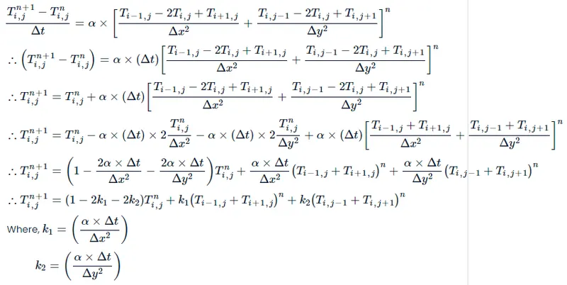
MATLAB code for unsteady explicit solver:-
Let us create code by considering above condition and equation.
clear all
close all
clc

L=1; %Length of square domain in meter
nx=ny=10; %Number of nodes (gridpoints)
%Mesh creation
x=linspace(0,L,nx);
dx=L/(nx-1); %Meshing in X direction
y=linspace(0,L,ny);
dy=L/(ny-1); %Meshing in Y direction

%2D matrix creation
[X,Y] = meshgrid(x,y);

%Initialization
T=300*ones(nx,ny);
T(:,1)=400; %Temperature at left wall
T(:,nx)=800; %Temperature at right wall
T(1,:)=600; %Temperature at top wall
T(ny,:)=900; %Temperature at bottom wall
T(1,1)=(400+600)/2; %Temperature at top left corner
T(nx,1)=(400+900)/2; %Temperature at bottom left corner
T(1,ny)=(600+800)/2; %Temperature at top right corner
T(nx,ny)=(800+900)/2; %Temperature at bottom right corner

alpha=1.4; %Diffusivity constant
dt=1e-3; %timestep value in seconds
t = 15; %Total time
nt = t/dt; %Number of timesteps
Told=T;
k1 = (alpha*dt)/(dx)^2 ;
k2 = (alpha*dt)/(dy)^2;
cfl = k1+k2; %Total cfl value, must be less than 0.5

tic;
%Time loop
for k=1:nt
  %Space loop
  for i=2:nx-1
    for j=2:ny-1
      T(i,j)=(1 - 2*k1 -2*k2)*Told(i,j) + k1*(Told(i-1,j)+Told(i+1,j)) + k2*(Told(i,j-1)+Told(i,j+1));
    endfor
   endfor
   %Reinitializing temperature values
   Told=T;
endfor

%Plotting
  figure(1)
  colormap(jet);
  [c,h] = contourf(x,y,T,'ShowText','on');
  set(gca,'YDIR','reverse');
  colorbar;
  title({'Transient state Explicit condition';['CFL ',num2str(cfl)]});
  xlabel('X co-ordinate');
  ylabel('Y co-ordinate');
  Ellapsed_time = toc
 %Ellapse time = 155.29 sec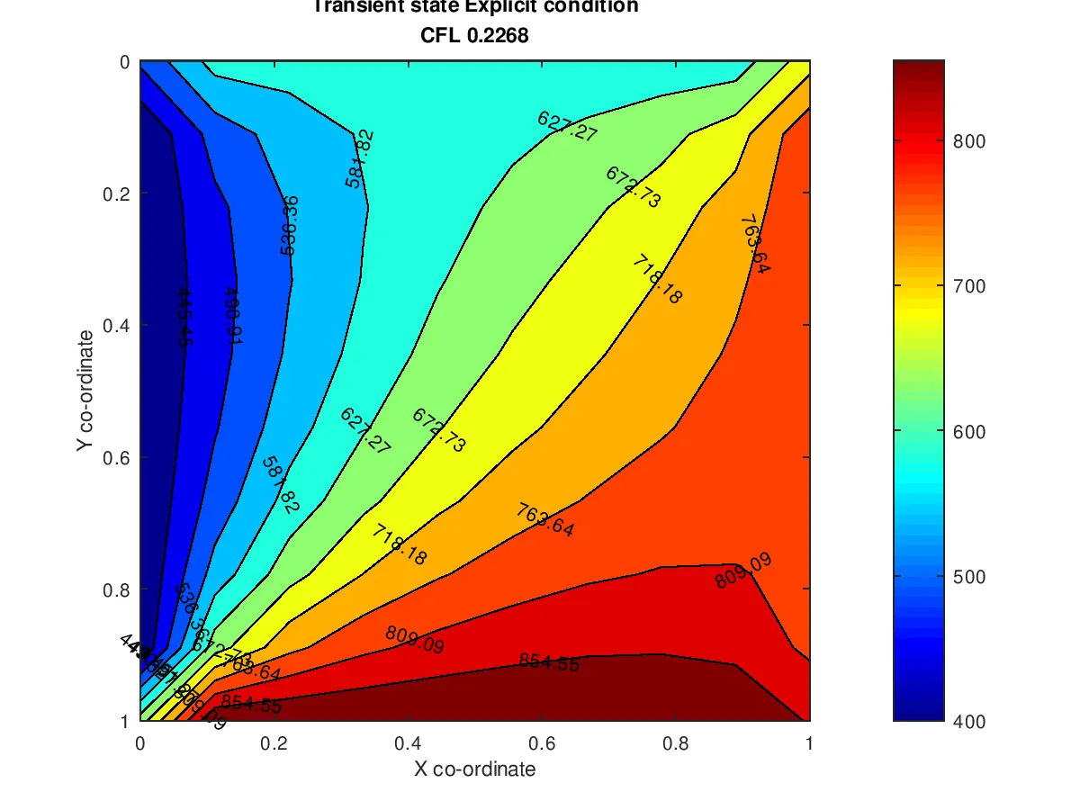
Above plot shows temperature profile by explicit solver. For transient explicit condition combined cfl value should be less than 0.5. If cfl value exceeds 0.5 then the solution will
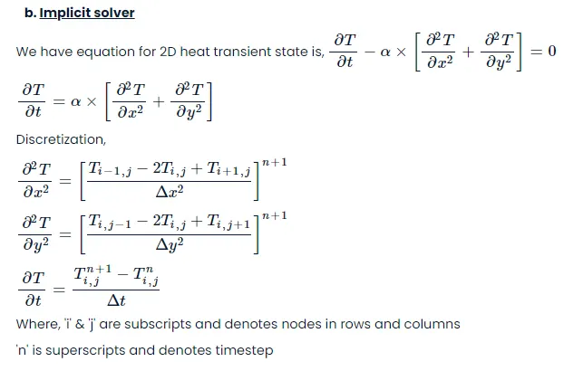
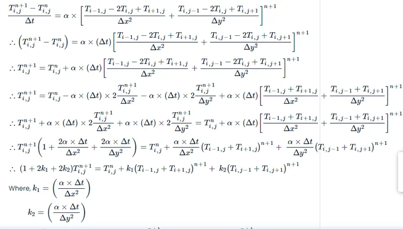
MATLAB code for unsteady implicit solver:-
Let us create code by considering above condition and equation.
clear all
close all
clc

L=1; %Length of square domain in meter
nx=ny=10; %Number of nodes (gridpoints)
%Mesh creation
x=linspace(0,L,nx);
dx=L/(nx-1); %Meshing in X direction
y=linspace(0,L,ny);
dy=L/(ny-1); %Meshing in Y direction

%2D matrix creation
[X,Y] = meshgrid(x,y);

%Initialization
T=300*ones(nx,ny);
T(:,1)=400; %Temperature at left wall
T(:,nx)=800; %Temperature at right wall
T(1,:)=600; %Temperature at top wall
T(ny,:)=900; %Temperature at bottom wall
T(1,1)=(400+600)/2; %Temperature at top left corner
T(nx,1)=(400+900)/2; %Temperature at bottom left corner
T(1,ny)=(600+800)/2; %Temperature at top right corner
T(nx,ny)=(800+900)/2; %Temperature at bottom right corner

alpha=1.4; %Diffusivity constant
dt=1; %timestep value in seconds
t = 15; %Total time
nt = t/dt; %Number of timesteps
Told=T;
Tprev=T;
k1 = (alpha*dt)/(dx)^2 ;
k2 = (alpha*dt)/(dy)^2;
k3 = (1+2*k1+2*k2)^(-1);
itr_jaco = 0;
itr_gs = 0;
itr_sor = 0;
tol=1e-4; %Convergence criteria

%Input method number
method= input('Enter method number 1.Jacobi 2.GS 3.SOR: ')

%Jacobian method
tic;
if method==1
  %Time loop
  for k=1:nt
    error=9e9; %Error reinitialization
    %Convergence loop
    while error > tol
      %Space loop
      for i=2:nx-1
        for j=2:ny-1
          T(i,j)= k3*Tprev(i,j) + k3*k1*(Told(i-1,j)+Told(i+1,j)) + k3*k2*(Told(i,j-1)+Told(i,j+1));
        endfor
      endfor

      error_n=abs(max(T-Told));
      error = max(error_n);
      Told=T; %Updating old values
      itr_jaco = itr_jaco + 1;
    endwhile
    Tprev = T; %Updating previous timestep values

    %Plotting
    figure(1)
    colormap(jet);
    [c,h] = contourf(x,y,T,'ShowText','on');
    set(gca,'YDIR','reverse');
    colorbar;
    xlabel('X coordinate');
    ylabel('Y coordinate');
    title(['Jacobian iteration value = ',num2str(itr_jaco)]);
    pause(0.01);
    %Ellapsed time = 46.163 sec
  endfor

%GS method
elseif method==2
%Time loop
  for k=1:nt
    error=9e9; %Error reinitialization
    %Convergence loop
    while error > tol
      %Space loop
      for i=2:nx-1
        for j=2:ny-1
          T(i,j)= k3*Tprev(i,j) + k3*k1*(T(i-1,j)+Told(i+1,j)) + k3*k2*(T(i,j-1)+Told(i,j+1));
        endfor
      endfor
      error_n=abs(max(T-Told));
      error = max(error_n);
      Told=T; %Updating old values
      itr_gs = itr_gs + 1;
    endwhile
    Tprev = T; %Updating previous timestep values

    %Plotting
    figure(2)
    colormap(jet);
    [c,h] = contourf(x,y,T,'ShowText','on');
    set(gca,'YDIR','reverse');
    colorbar;
    xlabel('X coordinate');
    ylabel('Y coordinate');
    title(['GS iteration value = ',num2str(itr_gs)]);
    pause(0.01);
    %Ellapsed time = 42.444 sec
  endfor

%SOR
elseif method==3
  %Time loop
  for k=1:nt
    error=9e9; %Error reinitialization
    %For w=0.8 no of iterations = 406
    %For w=0.9 no of iterations = 342
    %For w=1.0 no of iterations = 288
    %For w=1.1 no of iterations = 242
    %For w=1.2 no of iterations = 202
    %For w=1.3 no of iterations = 166
    %For w=1.4 no of iterations = 231
    %For w=1.5 no of iterations = 095
    %For w=1.6 no of iterations = 114
    %For w=1.55 no of iterations = 104
    %For w=1.51 no of iterations = 096
    %For w=1.49 no of iterations = 095
    %For w=1.48 no of iterations = 100

    w=1.495; %SOR over relaxation
    %Convergence loop
    while error > tol
      %Space loop
      for i=2:nx-1
        for j=2:ny-1
           Tgs= k3*Tprev(i,j) + k3*k1*(T(i-1,j)+Told(i+1,j)) + k3*k2*(T(i,j-1)+Told(i,j+1));
            T(i,j) = (1-w)*Told(i,j) + w*Tgs;
           endfor
      endfor
      error_n=max(abs(T-Told));
      error = max(error_n);
      Told=T; %Updating old values
      itr_sor = itr_sor + 1;
    endwhile
    Tprev = T; %Updating previous timestep values

    %Plotting
    figure(3)
    colormap(jet);
    [c,h] = contourf(x,y,T,'ShowText','on');
    set(gca,'YDIR','reverse');
    colorbar;
    xlabel('X coordinate');
    ylabel('Y coordinate');
    title(['SOR iteration value = ',num2str(itr_sor)]);
    pause(0.01);
    %Ellapsed time = 40.728 sec
  endfor
endif
 ellapsed_time=toc;
Above code consist of all 3 iterative solvers. When user enter 1 then code of Jacobian iterative solver starts running and display output on graph. Similarly, when user enter 2 then code for Gauss-Seidel iterative solver starts running and when user enter 3 then SOR code will run.
I. Jacobian solver
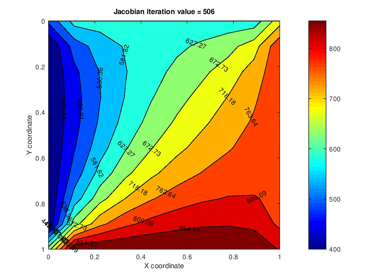 Above plot shows temperature profile by Jacobian solver. For solution convergence Jacobian solver required 506 iterations.
II. Gauss Seidel solver
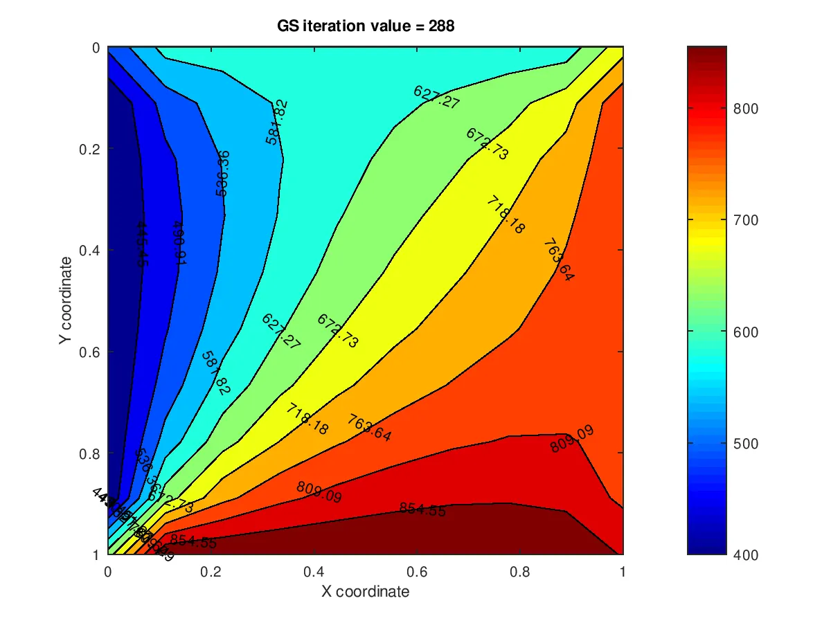
Above plot shows temperature profile by GS solver. For solution convergence this solver required 288 iterations.
III. SOR solver
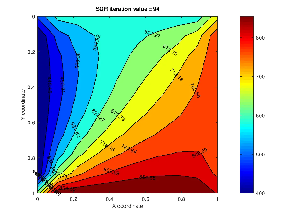
Above plot shows temperature profile by SOR solver. For solution convergence this solver required 94 iterations only. We get least number of iterations for ω=1.495ω=1.495.
| Jacobian solver | Gauss Seidel solver | SOR solver | |
| Number of iterations required to converge solution for steady State equation | 208 | 112 | 24 |
| Number of iterations required to converge solution for transient State implicit equation | 506 | 288 | 94 |
| Time elapsed to converge solution for steady State equation (Second) | 542.28 | 382.46 | 102.00 |
| Time elapsed to converge solution for transient State implicit equation (Second) | 46.163 | 42.444 | 40.728 |
| Table: Comparison of iterations and time elapsed for converging solution for iterative solvers | |||