Project 1
Aim
a. Tabulate the fuel economy numbers (kmpl) for UDDS and HWFET cycle. This forms the baseline numbers for comparing with the future hybrid version.
b. Plot the time trace for engine, transmission input, transmission output and wheel speed on one plot.
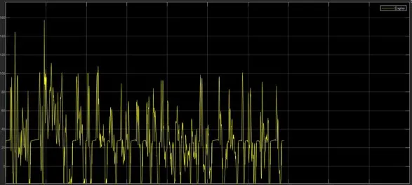
c. Plot engine torque, engine power, fuel rate and fuel consumption using subplots.
d. Plot accelerator and brake pedal, gear command, vehicle desired and actual speed, vehicle distance using subplots.
e. Plot the engine operating points on the engine fuel map.
f. Write down appropriate brief comments on each of these plots, describing the vehicle behavior throughout the drive cycle.
g. Generate the plots for both drive cycles
Theory
Ordinary Vehicle:
Traditional vehicles utilize a gas powered motor energized by fuel or diesel to drive the wheels. In this the intensity motor purposes the rule of intensity discharge through ignition of a fuel with an oxidizer in a burning chamber to make growing gases which pushes against a cylinder making forcce and force yield.
In this vehicle motor proselytes compound energy put away in the fuel into heat which is utilized to deliver helpful work. Regularly utilize non-renewable energy sources like petrol (petroleum and diesel).
The most well known sort of motor is utilized in this framework is 4 stroke responding motor. Motor in cyclinder interaction can be addressed by ideal thermodynamic cycles, for example, Otto cycle, Diesel cycle. Otto cycle is an ideal cycle thet depicts the cycle interaction for flash lighted SI motor. furthermore, the Diesel cycle is the ideal cycle thet portrays the cycle interaction for a pressure lighted Cl motor.
Energy and execution of vehicle:
In this framework trge power interest on the wheel need to moment provided by the powertrain. In otyher word the power coming from the powertrain directs the power interest on the wheels (according to execution viz, speed increase, speed and so still up in the air by it.
In tis vehicle the powertrain is comprises of a motor associated with the wheels through a transmission thusly the power comes from the motor through the transmission.
Framework Dynamics:
It manages the displaying of multi space frameworks using a brought together methodology in light of a customary differential and mathematical condition depicting the static and dynamic impacts.
Every frameworks has are two summed up factors
1] Efforts:- It is summed up force variable. ex-force, force, voltage, warming worth.
2] Flow: It is the summed up stream/speed variable. ex:- speed, current, mass stream rate.
3] Power:- It is the result of the work and stream variable. It is exchangeable between energy areas.
`m_f=(P_e)/(eta_e*eta_t*QLHV)`
mf=mass flow rate
pe=power of transmission
nt=efficiency of transmission
ne=efficiency of engine
QHLV=Calorific value
Energy based models-Element models
To models the inside actual properties of the component and the misfortunes there are essentially two sorts of approach.
1] Map based models:- Elements are demonstrated utilizing maps which described the connection between the info and result, result and misfortunes and so forth.
2] Analytical models:- Elements are demonstrated utilizing actual condition that address the inner elements. These are the two limits most models are a mix of the two for certain elements models systematically and for some utilizing maps.
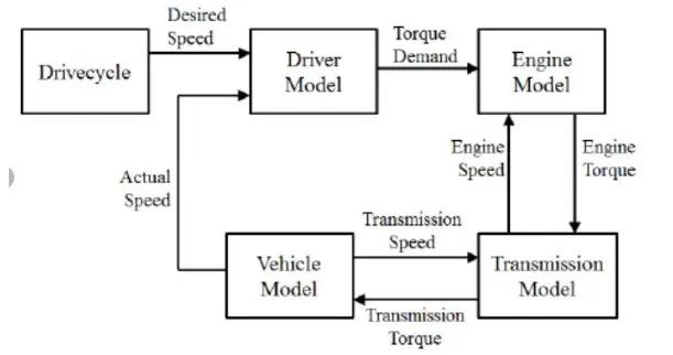
Matlab script
Run this script first
%%%%%%%%%%%%%%%%%%%%%%%%%%%%%%%%%%%%%%%%%%%%%%%%%%%%%%%%%%%%%%%%%%%%%

Skill-Lync -> Hybrid Drives Development
Project 1 - Conventional Vehicle Model By - Joseph
% Description:

Initialization File
Initialization file for loading the variables for the Conventional vehicle simulation model
Vehicle Parameters
M = 1500;       % Vehicle weight [kg]
Cr = 0.015;     % Rolling resistance coefficient
Rw = 0.35;      % Rolling radius [m]
Cd = 0.33;      % Drag coefficient
Af = 2;         % Frontal area [m2]
rhoa = 1.225;   % Air density [kg/m3]
Vwind = 0;      % Wind velocity [kmph]
g = 9.81;       % Gravitational acceleration [m/s2]
theta = 0;      % Slope [deg]
myu_road_tire = 1; % Coefficient of friction between tire - road interface

Powertrain Parameters
FDR = 3.73;                         % Final Drive Ratio / Diff Ratio
DiffEff = 0.99;                     % Differential efficiency (assumed independent of operating conditions)

NumGear = 4;                        % Number of gears in transmission
TransGear = [1:NumGear];            % Transmission Gears
TransRatio = [3.06, 1.62, 1, 0.7];  % Corresponding Transmission ratios
TransEff = 0.90;                    % Transmission efficiency (assumed independent of operating conditions)

TC_SR = [0, .5, .6, .7, .8, .87, .92, .94, .96, .97, 1];   % Torque Converter Speed Ratio (Matlab default) -> TurbSpd/PumpSpd
TC_TR = [2.232, 1.5462, 1.4058, 1.2746, 1.1528, 1.0732, 1.0192, 1, 1, 1, 1];   % Torque Converter Torque Ratio (Matlab default) -> TurbTrq/PumpTrq
TC_Cf = 1e-4 * [.72558, .66322, .63463, .59042, .51331, .4144, .29287, .22444, .12186, .04386, 0]; % Torque Converter Capacity Factor (Matlab default) -> PumpTrq/PumpSpd^2 [Nm/rpm^2]

load Vehicle_Data/Engine_data_1_9L_Saturn_95kW
load Vehicle_Data/Trans_Shift_map

Driver Parameters
Kp = 10;                    % P gain for driver PI model
Ki = 1;                     % I gain for driver PI model
Drive_Cycle_Select = 1;     % Drive cycle selection

% Drive cycle values in m/s

if Drive_Cycle_Select == 1
    load DriveCycles/UDDS;

elseif Drive_Cycle_Select == 2
    load DriveCycles/HWFET;

elseif Drive_Cycle_Select == 3
    load DriveCycles/FTP;

elseif Drive_Cycle_Select == 4
    load DriveCycles/US06;

elseif Drive_Cycle_Select == 5
    load DriveCycles/NEDC;

elseif Drive_Cycle_Select == 6
    load DriveCycles/WLTP;

end

time_end = cyc_time(end);
vel_end = cyc_vel(end);
In this model We use Forward Model:
It otherwise called dynamic reproduction. Dynamic models are utilized for definite recreations. In this model power/force/power is the information and the vehicle state variable speed and speed increase are yields. The models and simulatios are more practical due to phhysical loss thus suitable for control advancement. There is criticism circle to meet the ideal vehicle state. It is principally used to reenact a vehicle on a driving cycle to dissect the powerful way of behaving of the framework helps fundamentally in charge improvement.
Modifications in simulink
Engine
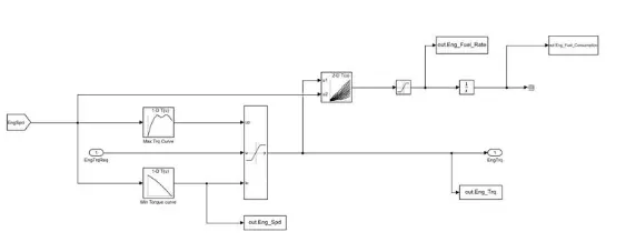
Driver Model graph
Vehicle Dynamics
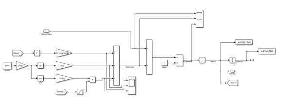
Governing Equation
`M_e((dV_v)/dt)=((eta_t*lambda_t)/(Rw))T_m- 1/2*A*c_d*(V_v+V_w)^2+C_r*M*g*cos(theta)+M*g*sin(theta)`
p=air density
A=Frontal Area
Cd=Drag Coefficient
Vveh=Velocity of vehicle
Vwind=velocty of wind
Cr=Rolling resistance
M=mass
g=gravity
Result
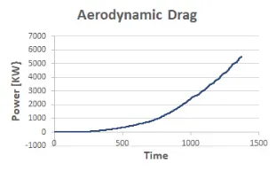
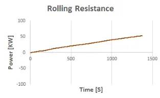
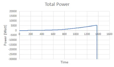
UDDS cycle
Conclusion
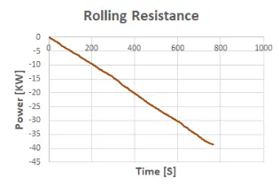
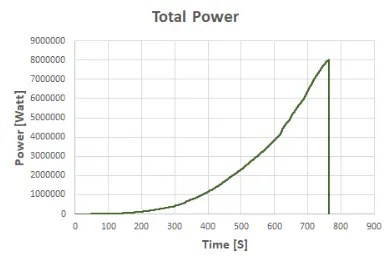
When rolling resistance,aerodynamic drag and inertial resistance increases total powe also increases
HWFET Cycle
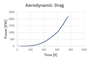
Result
Best is UDDS cycle