Project 1
Aim
- To use toposheet for catchment area calculations.
- To calculate flow for selected river using UH Method
- To analyse and observe differnt run profiles and steady flow analysis
Software Required
- Microsoft Excel
- HEC-RAS
- Autocad
- Google Chrome (Or any other browser)
- Google Earth Pro
Procedure
- Select a river. Here I choose narmada river.
- Consider minimum of 10km river reach.
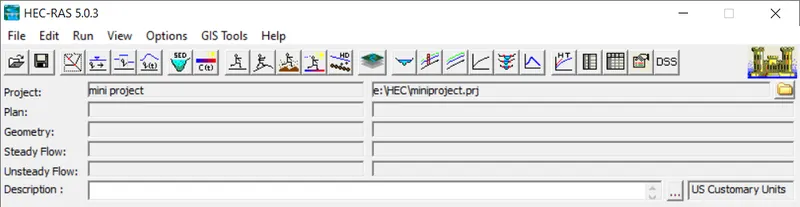
- Start a new project in HEC-RAS software.
- Open cross section data editor and give the necessory values.
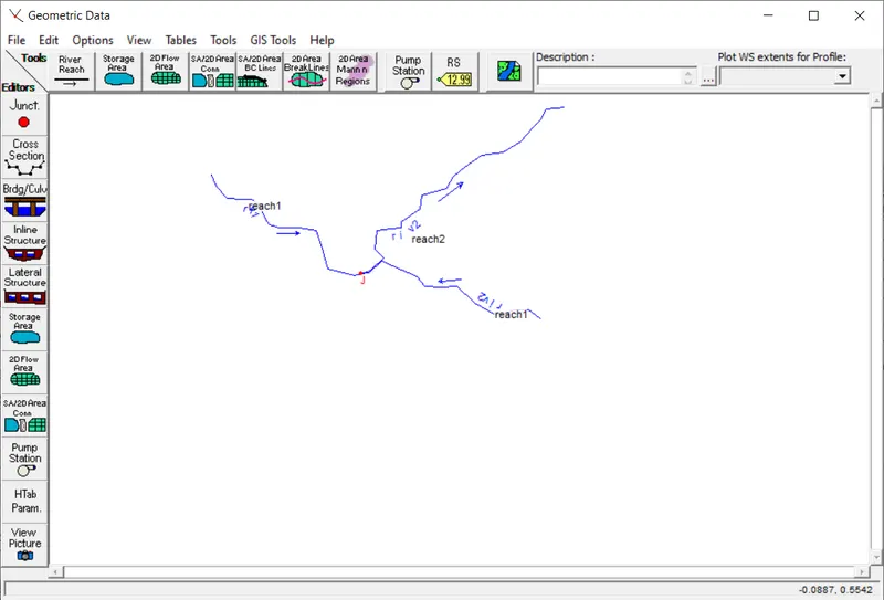
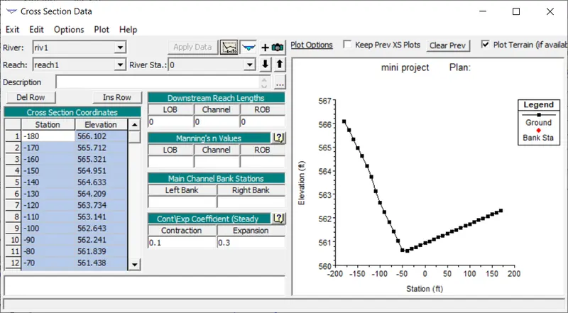
- Click Options -> Add cross section data.
- Change river station to a value and change the necessory data required.
- Similarly,add all data of cross section of each station and then click on 'apply data' option to get a graph plotted on the right side of that window.
- Click on plot -> plot profile to view that.
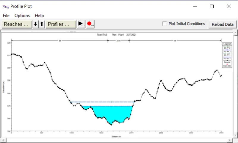
- Then click on file menu -> save geometry data as option.
- Then save the cross section data in appropriate folder.
- Now we can move to the section of catchment area calculation.
- Open Google Chrome (or any other browser)
- Search for "SOI Nakshe".
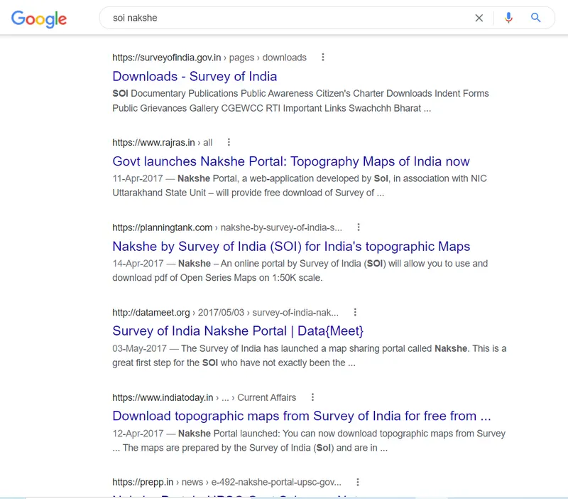
- Select the link which direct to the site "https://onlinemaps.surveyofindia.gov.in/"
- A home page will appear then.
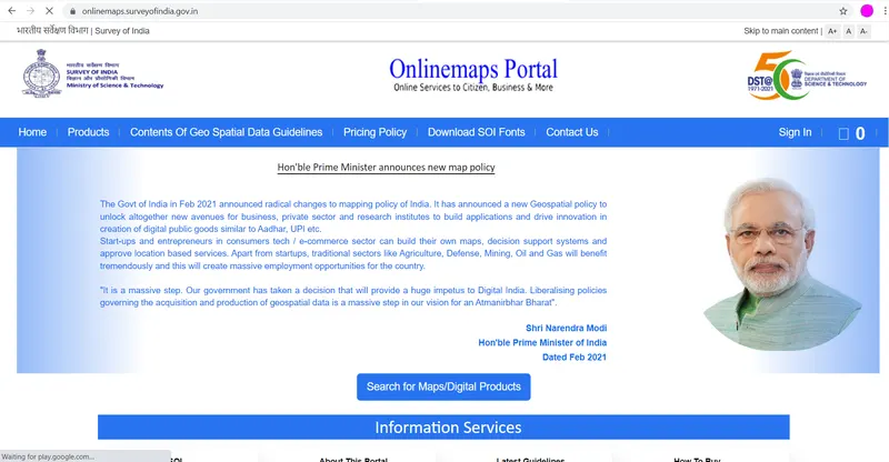
- Click on Sign In.
- Then a box will appear for signing in.
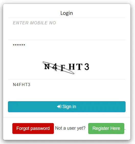
- If its a first ttime user, then click on "Register Here" option. Then register with an email id and enter a password.
- Then an OTP will come at your registered email id.
- After reading all the terms and condition, do the needful.
- Else Enter Mobile Number, Password and Captcha.
- Then click Sign In.
- After successful login a new screen will appear with online toposheet series.
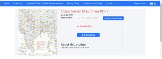
- Enter the toposheet number and click download button.
- Then a pdf will get download.
- Convert it into .jpg format in order to insert this image into the Autocad Software.
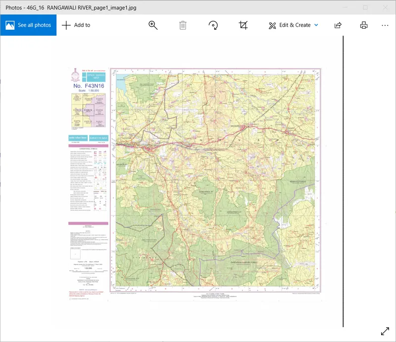
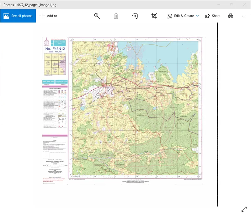
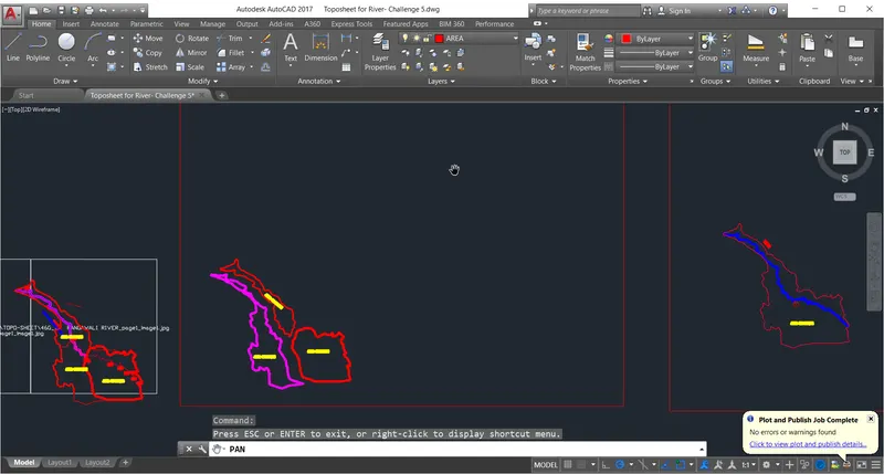
- Then open it in Autocad.
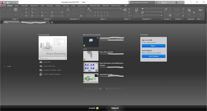
- Click start Drawing option.
- Click File -> Import -> PDF (or .jpg).
- The image will appear on screen.
- Considering it as a background image, draw the necessary data needed in an another layer.
- Then sketch the layout of river using the polyline tool
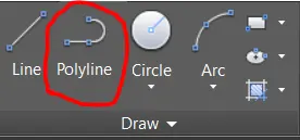 which is under draw option in home tab.
 - Click Area
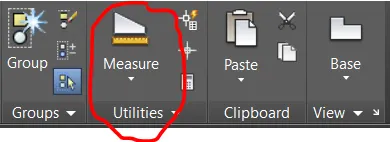
- Then click on the boundary upto which area is to be known.
- Then area will be shown there.
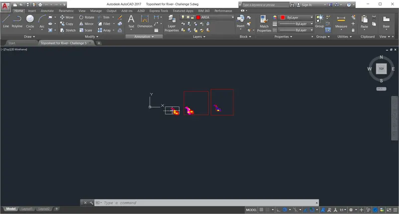
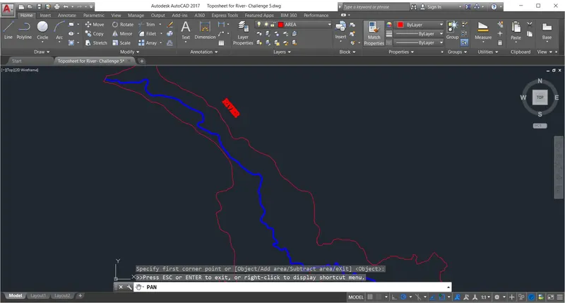
- Like that any area can be calculated here accuratly.
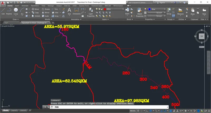
- Each river can again be selected clicking on the line itself. And deselect by pressing esc key on the keyboard.
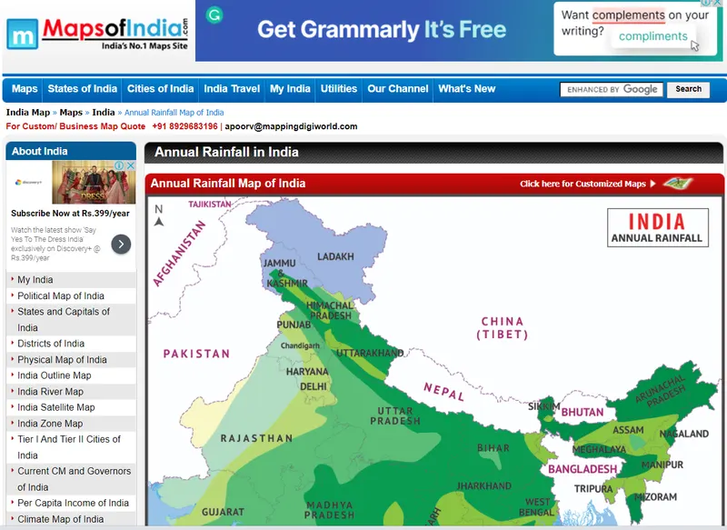
- To get isopluvial map go to website https://www.mapsofindia.com/maps/india/annualrainfall.htm
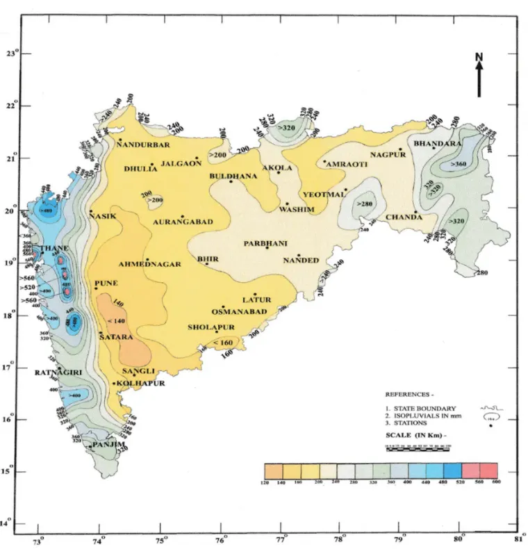
- Collect the isopluvial map for flood after 25 year from wesite.
- Also collect the isopluvial map for flood after 100 year from wesites.
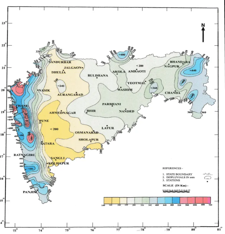
- Plot these data obtained in a table.
-
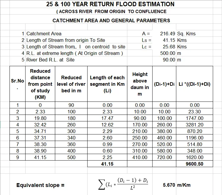
1 Catchment Area A = 216.49 Sq. Kms 2 Length of Stream from origin To Site Ls = 41.15 Kms 3 Length of Stream from I on centroid to site Lc = 25.68 Kms 4 R.L. at extreme length ( At Origin of Stream ) 500.00 m 5 River Bed R.L. at Site 90.00 m -
Sr.No. Reduced distance from point of study (KM) Reduced level of river bed in m Length of each segment in Km (Li) Height above datum in m 1 0 90 0.00 0.00 2 2.33 100 2.33 10.00 3 19.80 180 17.47 90.00 4 32.42 260 12.62 170.00 5 34.71 300 2.29 210.00 6 37.31 340 2.60 250.00 7 38.30 360 0.99 270.00 8 38.90 400 0.60 310.00 9 41.15 500 2.25 410.00 - Find Equivalent stream slope (S) using analytical method. Add 2 more column [(Di-1)+Di] and [Li *((Di-1)+Di)] for that.
- `S=Sigma((Li⋅(Di-1)+Di)/L^2)`
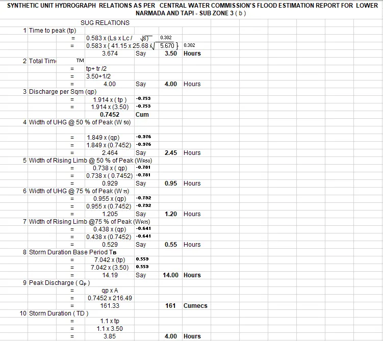
- Find the synthetic unit hydrograph datas using equations.
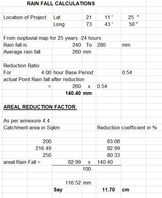
- Now calculate rainfall of 25 years.
- Calculate the time distribution of cumulative Hourly Rainfall (i.e. 25 year rainfall excess)
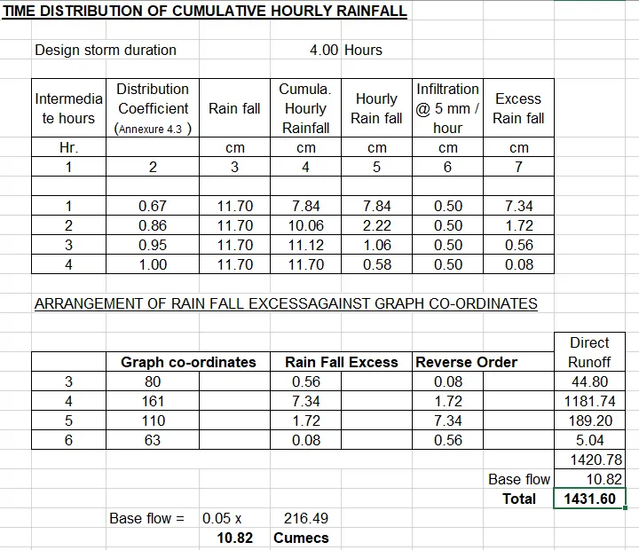
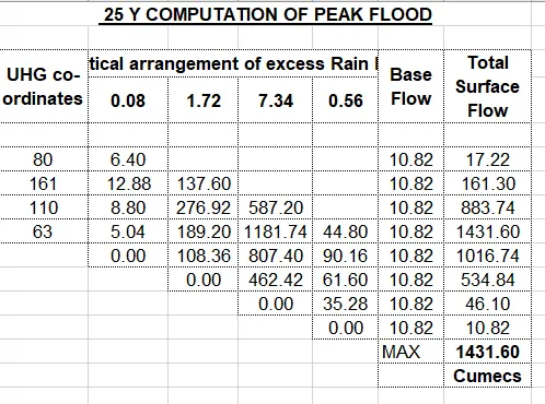
- Then compute 25 years of peak flood.
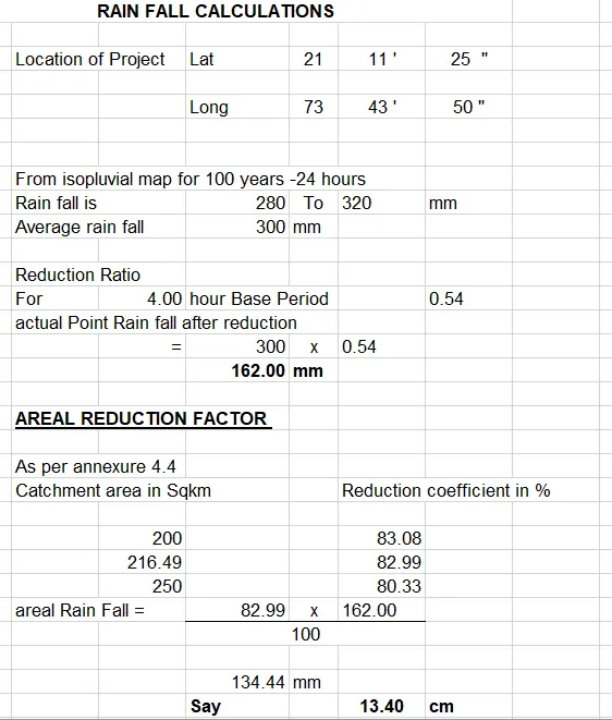
- Similarly calculate the rainfall calculations for 100 years.
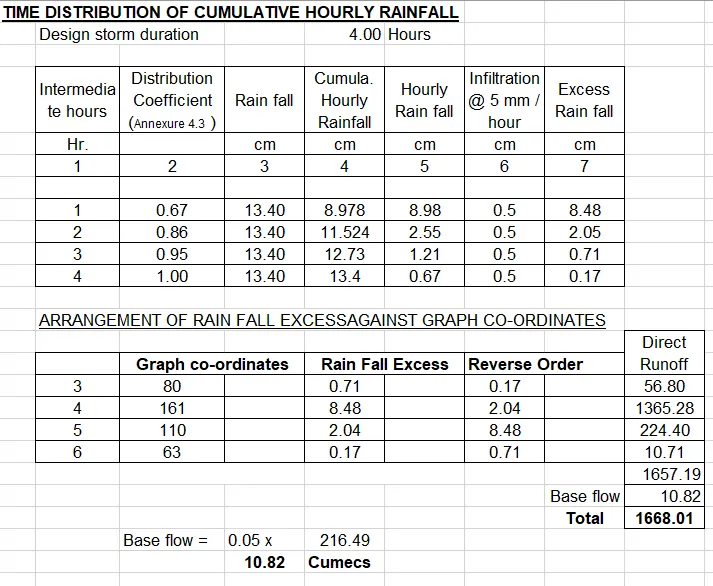
- Calculate the time distribution of cumulative Hourly Rainfall (i.e. 100 year rainfall excess)
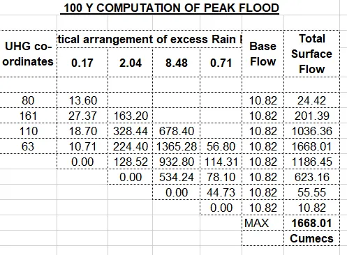
- Then compute 100 years of peak flood.
- Then plot a graph with the following datas
Time (Hours) Discharge (Cumecs) 0 0 1 12 2 36 3 80 4 161 5 110 6 63 7 44 8 32 9 23 10 16 11 11 12 6 13 3 14 0 ∑ 597 - Graph is plotted time in x axis and discharge in y axis.
- Maximum Discharge is 161 cumecs
- A check can also be done to know whether the obtained result is right or not using the equation, `(ΣQ⋅3600⋅100)/(C⋅A⋅10^6)`
- Now we can move on to the steady flow analysis section.
- Click on 'Perform a Steady flow simulation' on the main window for steady flow analysis.
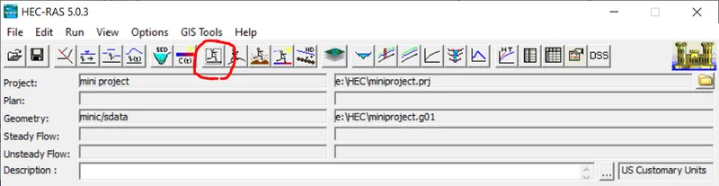
- This component of the modeling system is intended for calculating water surface profiles for steady gradually varied flow. The system can handle a full network of channels, a dendritic system, or a single river reach. The steady flow component is capable of modeling subcritical, supercritical, and mixed flow regimes water surface profiles.
The basic computational procedure is based on the solution of the one-dimensional energy equation. Energy losses are evaluated by friction (Manning's equation) and contraction/expansion (coefficient multiplied by the change in velocity head). The momentum equation may be used in situations where the water surface profile is rapidly varied. These situations include mixed flow regime calculations (i.e., hydraulic jumps), hydraulics of bridges, and evaluating profiles at river confluences (stream junctions). 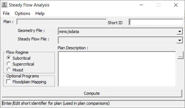 (By clicking on compute, we can see if there is any errors. If so a pop up window will appear showing what are the absent values for the correct processing of data.)
- Then click on set locations for flow distribution option for entering various datas.
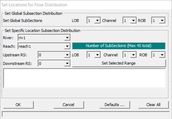
- Also click on Add Flow Change Location button and Add Multiple button when necessory.
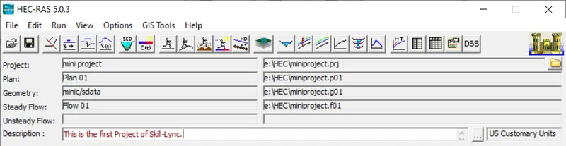
- Click file menu -> Save to save the entire steady flow calculations.
- Then the main window will be like this,
Result
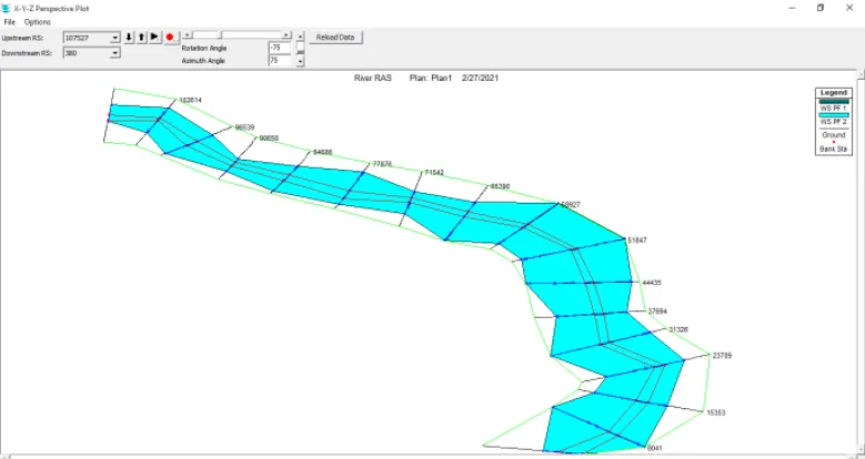 The final result of cross section can be checked in X-Y-Z Perspective Plot option of HEC-RAS software.
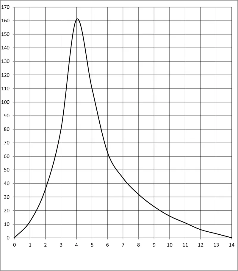 Flood estimation for 25 years and 100 years are calculated using UH method. And analysis is done and graph is plotted and check is done.
- Run model of different profiles are plotted.
- Steady flow analysis also done.