Project 1

AIM:

The task of this project is to compute the fuel economy numbers for the given vehicle (kmpl) on the urban cycle (UDDS) and highway cycle (HWFET). Also, to analyze and understand the vehicle operating
points in terms of engine speed, torque, transmission speeds, pedal positions, gear, distance traveled, etc.

OBJECTIVES:

1. Tabulate the fuel economy numbers (kmpl) for UDDS and HWFET cycle. This forms the baseline numbers for comparing with the future hybrid version.
2. Plot the time trace for engine, transmission input, transmission output and wheel speed on one plot.
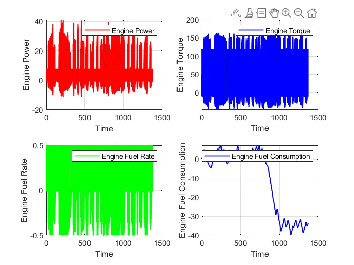
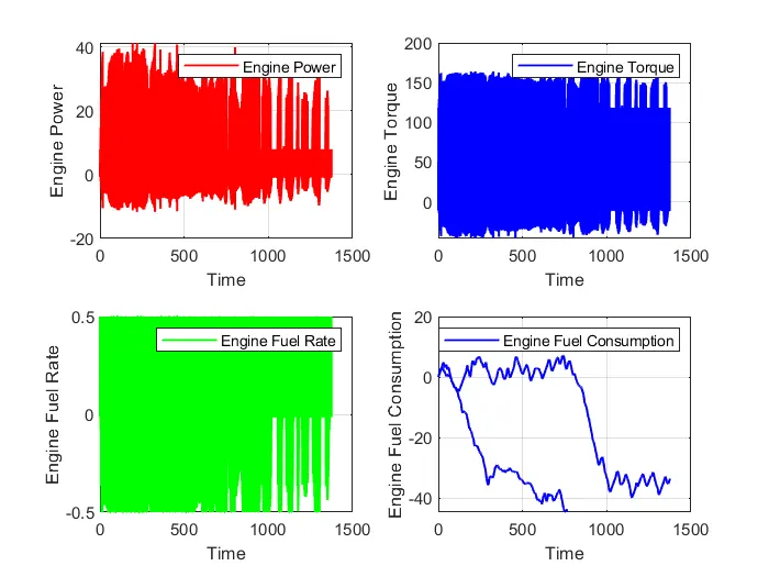
3. Plot engine torque, engine power, fuel rate and fuel consumption using subplots.
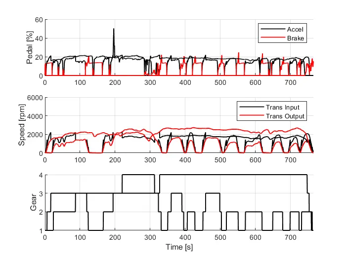
4. Plot accelerator and brake pedal, gear command, vehicle desired and actual speed, vehicle distance using subplots.
5. Plot the engine operating points on the engine fuel map.
6. Write down appropriate brief comments on each of these plots, describing the vehicle behavior throughout the drive cycle.
7. Generate the plots for both drive cycles

THEORICITAL CONCEPTS REGARDING FORWARD ENERGY MODEL OF CONVENTIONAL VEHICLE:

A driver controller is required to control the vehicle to follow a desired speed and set the start of the calculations. The controller is implemented to model the driver that will either push the accelerator or the brake pedal to match the desired speed which enables to study the driver behaviour. The controller is used as part of a feedback loop that will determine the energy required to drive the vehicle.

Vehicle Energy Consumption Estimation Models

• Analytical models:

  Analytical models are representative of the Vehicle behaviour and can be developed in MATLAB/Simulink by creating an vehicle model. They are based on fundamental theoretical equations. A model of the vehicle dynamics is built based on vehicle dynamics theory to calculate the power required at the wheels to overcome the resistances forces opposed to the vehicle motion: Aerodynamic Drag, Rolling, Inertia, Gradient and Transmission resistances. The power required derives from the tractive force expressed as the sum of the resistances forces above

• Statistical models:

  Statistical models are built based on real world driving data analysis to derive empirical relationships between the different factors affecting Vehicles energy consumption.

• Computational models:

  There are mainly two kinds of computational models for energy consumption estimation: Artificial Neural Networks (ANN) based model. Clustering based models

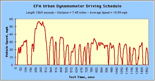
UDDS Cycle: The EPA Urban Dynamometer Driving Schedule (UDDS) is commonly called the "LA4" or "the city test" and represents city driving conditions. It is used for light duty vehicle testing. The UN/ECE Regulation 53 refers to the EPA UDDS as the "Test Equivalent to the Type 1 Test (verifying emissions after a cold start)."

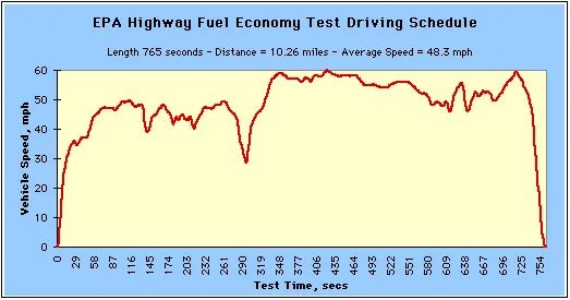
HWFET Cycle: The Federal Test Procedure (FTP) is composed of the UDDS followed by the first 505 seconds of the UDDS. It is often called the EPA75. The dynamometer portion of the test procedure has a very complex timeline of events.

Model

Initial Matlab Model: “Project1_InitFile.m” ( For UDDS cycle & HWFET cycle)

close all
clear all
clc

% Skill-Lync -> Hybrid Drives Development
% Project 1 - Conventional Vehicle Model
% By - Ankit Kumar Singh 

% Description:

%% Initialization File
% Initialization file for loading the variables for the Conventional vehicle simulation model

% Vehicle Parameters
M = 1500;                           % Vehicle weight [kg]
Cr = 0.015;                         % Rolling resistance coefficient
Rw = 0.35;                          % Rolling radius [m]
Cd = 0.33;                          % Drag coefficient
Af = 2;                             % Frontal area [m2]
rhoa = 1.225;                       % Air density [kg/m3]
Vwind = 0;                          % Wind velocity [kmph]
g = 9.81;                           % Gravitational acceleration [m/s2]
theta = 0;                          % Slope [deg]
myu_road_tire = 1;                  % Coefficient of friction between tire - road interface

%% Powertrain Parameters 
FDR = 3.73;                         % Final Drive Ratio / Diff Ratio
DiffEff = 0.99;                     % Differential efficiency (assumed independent of operating conditions)

NumGear = 4;                        % Number of gears in transmission
TransGear = [1:NumGear];            % Transmission Gears
TransRatio = [3.06, 1.62, 1, 0.7];  % Corresponding Transmission ratios
TransEff = 0.90;                    % Transmission efficiency (assumed independent of operating conditions)

TC_SR = [0, .5, .6, .7, .8, .87, .92, .94, .96, .97, 1];   % Torque Converter Speed Ratio (Matlab default) -> TurbSpd/PumpSpd  
TC_TR = [2.232, 1.5462, 1.4058, 1.2746, 1.1528, 1.0732, 1.0192, 1, 1, 1, 1];   % Torque Converter Torque Ratio (Matlab default) -> TurbTrq/PumpTrq
TC_Cf = 1e-4 * [.72558, .66322, .63463, .59042, .51331, .4144, .29287, .22444, .12186, .04386, 0];                         % Torque Converter Capacity Factor (Matlab default) -> PumpTrq/PumpSpd^2 [Nm/rpm^2]

load Vehicle_Data/Engine_data_1_9L_Saturn_95kW
load Vehicle_Data/Trans_Shift_map

%% Driver Parameters
Kp = 10;                             % P gain for driver PI model
Ki = 1;                              % I gain for driver PI model
Drive_Cycle_Select = 1;              % Drive cycle selection

% Drive cycle values in m/s

if Drive_Cycle_Select == 1
    load DriveCycles/UDDS;
    
elseif Drive_Cycle_Select == 2
    load DriveCycles/HWFET;
    
elseif Drive_Cycle_Select == 3
    load DriveCycles/FTP;
    
elseif Drive_Cycle_Select == 4
    load DriveCycles/US06;
    
elseif Drive_Cycle_Select == 5
    load DriveCycles/NEDC;
    
elseif Drive_Cycle_Select == 6
    load DriveCycles/WLTP;
 
end

time_end = cyc_time(end);
vel_end = cyc_vel(end);

The Simulink Model -

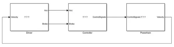
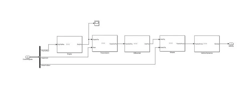
this model has threeblocks Driver, Controller and Powertrain . there are 2 empty sub blocks in powertrain the Engine sub-block and Vehicle Dynamics.

they had created acc to given initial file data . after simulated these 'To workspace' blocks used those data from initial file data.

Driver Block:

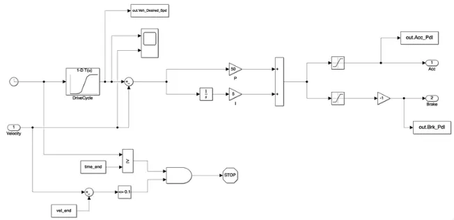
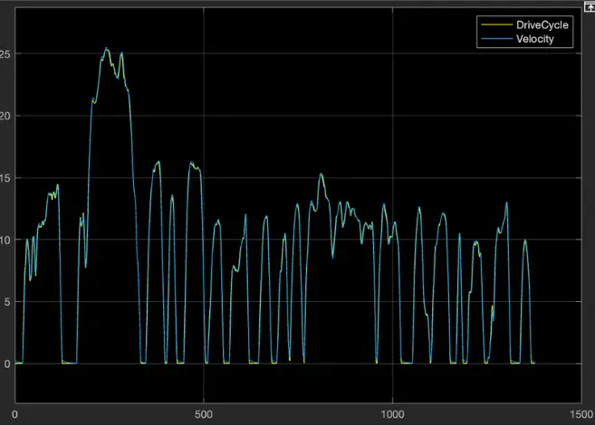
Drive Cycle and Velocity (Scope): For UDDS cycle

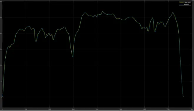
Drive Cycle and Velocity (Scope): For HWFET cycle

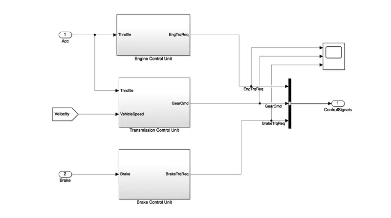
Controller Block:

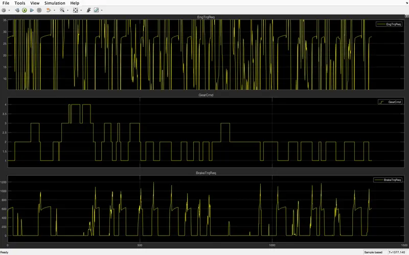
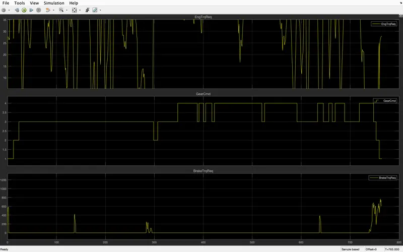
Engine Torque Required, Gear command, Brake Torque Required (Scope): UDDS cycle

Engine Torque Required, Gear command, Brake Torque Required (Scope): HWFET cycle

Powertrain Block:

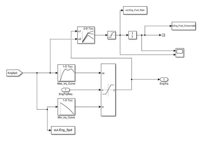
Engine:

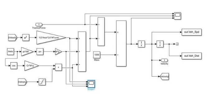
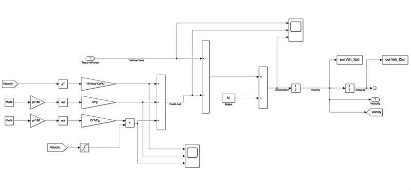
Now, the Vehicle dynamics block is developed using the equations
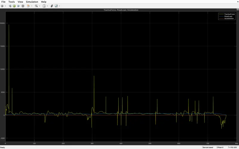
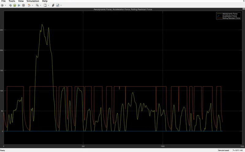
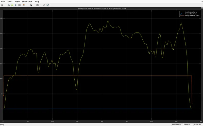
Equations for aerodynamic drag, rolling resistance, and gradient are created and summed up to get the road load
Road load is subtracted from the tractive force to get the force
This force is then divided by the mass to get the acceleration component
Integrator is used to integrate the acceleration and get the velocity component
Road load and velocity are multiplied to get the power required for the vehicle
Power is then multiplied by the total time to get the energy required
All the blocks of velocity, acceleration, road load, the power required, and energy required are attached to the 'scope' block to
see the output variations with respect to the time

Vehicle Dynamics:

Transmission Block:

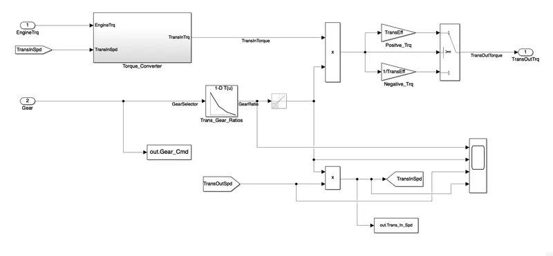
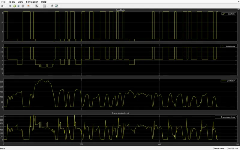
Gear ratio, Ratio limiter, Transmission input speed and transmission output speed: For UDDS cycle

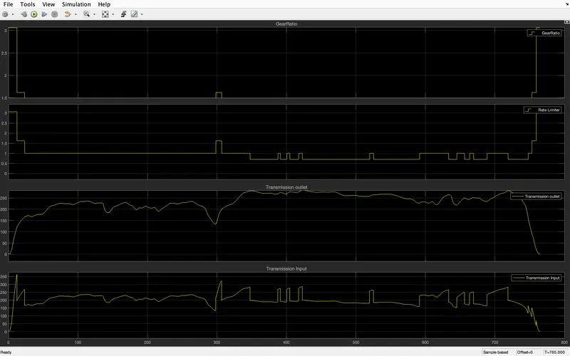
Gear ratio, Ratio limiter, Transmission input speed and transmission output speed: For HWFET cycle

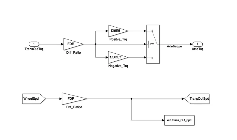
Differential block:

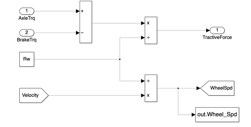
Wheel Block:

Vehicle Dynamics Block:

Tractive Force, Road Load and Acceleration : For UDDS cycle

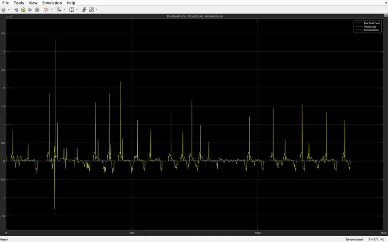
Tractive Force, Road Load and Acceleration : For HWFET cycle

Aerodynamic Force, Acceleration force, Rolling ressistance force: For UDDS cycle

Aerodynamic Force, Acceleration force, Rolling ressistance force: For HWFET cycle

Code for 'Project1_ProcessingFile -

% Skill-Lync -> Hybrid Drives Development
% Project 1 - Conventional Vehicle Model
% By - Ankit Kumar Singh

% Description:
% The following file is to used with the Initialization file and Simulink
% results for post-processing of the data.
% The file is incomplete, has some examples of how the data is imported
% into a readable format, data analysis and plotting examples.
% Based on the project task, use commands in a similar format as given
% below, to analyse the data and generate required plots.
% You can change variable names if desired

% Post-Processing File
% File for post-processing the Conventional vehicle simulation model data

% Renaming variables
Time = out.tout;
Acc_Pdl = out.Acc_Pdl;                  % Accelerator pedal [%]
Brk_Pdl = out.Brk_Pdl;                  % Brake pedal [%]
Gear_Cmd = out.Gear_Cmd;                % Transmission gear
Trans_In_Spd = out.Trans_In_Spd*30/pi;  % Transmission input speed [rpm]
Trans_Out_Spd = out.Trans_Out_Spd*30/pi;% Transmission output speed [rpm]
Eng_Trq = out.Eng_Trq;                  % Engine brake torque [Nm]
Eng_Spd = out.Eng_Spd*30/pi;            % Engine speed [rpm]
Eng_Fuel_Consump = out.Eng_Fuel_Consumption;    % Engine fuel consumption [g]
Veh_Dist = out.Veh_Dist/1000;           % Distance traveled by vehicle [km]
Veh_Spd = out.Veh_Spd*18/5;             % Vehicle speed [kmph]
Wheel_Spd = out.Wheel_Spd;              % Wheel speed [kmph]
Eng_Fuel_Rate = out.Eng_Fuel_Rate;      % Engine Fuel Rate [%]
Veh_Desired_Spd = out.Veh_Desired_Spd;  % Vehicle Desired Speed [kmph]

%% Data Analysis
Eng_Pwr = Eng_Spd*pi/30*Eng_Trq/1000;   % Engine brake power [kW]
rho_petrol = 0.7197;                    % Density of petrol [kg/L]
kmpl = Veh_Dist(end)/(Eng_Fuel_Consump(end)/1000/rho_petrol);    % Fuel economy [kmpl] 


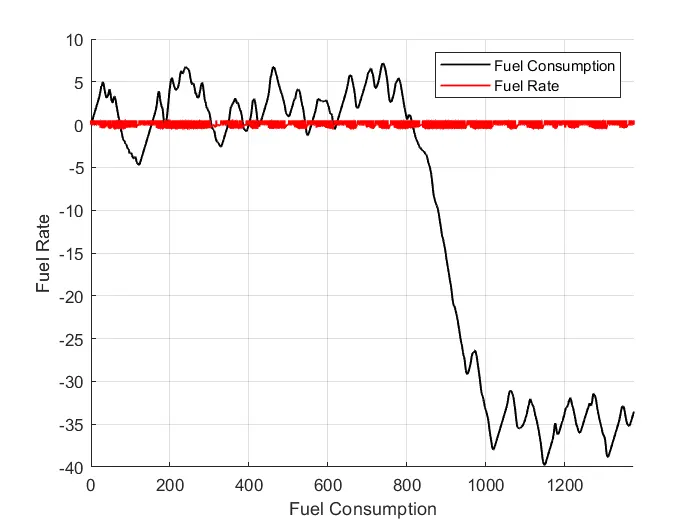
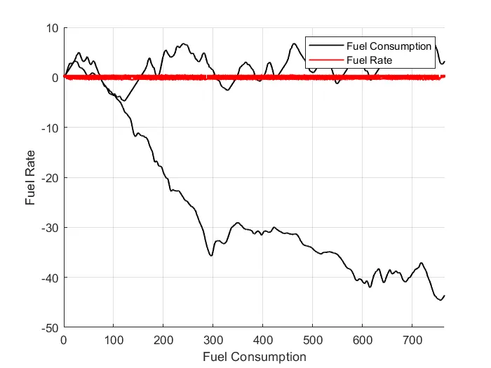
%% Plotting fuel consumption vs fuel rate
figure (1)
hold on
grid on
plot (Time,Eng_Fuel_Consump.data,'linewidth',2);    % Engine Fuel Consumption
plot (Time,Eng_Fuel_Rate.data,'linewidth',2);       % Engine Fuel Rate
xlabel ('Fuel Consumption');
ylabel ('Fuel Rate');
xlim ([0, Time(end)]);
legend ('Fuel Consumption','Fuel Rate');

%% Plotting vehicle characteristics time trace, engine, transmission input, transmission output and wheel speed on one plot
figure (2)
hold on 
grid on
plot (Time,Eng_Spd.data,'linewidth',2);         % Engine Speed 
plot (Time,Trans_In_Spd,'linewidth',2);         % Transmission Input
plot (Time,Trans_Out_Spd,'linewidth',2);        % Transmission Output
plot (Time,Wheel_Spd.data,'linewidth',2);       % Wheel Speed
xlabel ('Time [s]');
ylabel('Speed [rpm]')
xlim([0, Time(end)]);
legend('Engine Speed','Transmission Input','Transmission Output','Wheel Speed');

%% Plot engine torque, engine power, fuel rate and fuel consumption using subplots
% Engine Torque
figure (3)
subplot (2,2,1)
hold on
grid on
plot (Time,Eng_Trq.data,'linewidth',2);         % Engine Torque
xlabel ('Time [sec]');
ylabel ('Torque [Nm]');
legend ('Torque');
% Engine Power
subplot (2,2,2)
hold on
grid on
plot (Time,Eng_Pwr.data,'linewidth',2);         % Engine Power
xlabel ('Time [sec]');
ylabel ('Power [kW]');
legend ('Power');
% Engine Fuel Rate
subplot (2,2,3)
hold on
grid on
plot (Time,Eng_Fuel_Rate.data,'linewidth',2);   % Engine Fuel Rate
xlabel ('Time [sec]');
ylabel ('Fuel Rate [%]');
legend ('Fuel Rate');
% Engine Torque
subplot (2,2,4)
hold on
grid on
plot (Time,Eng_Trq.data,'linewidth',2);         % Engine Torque
xlabel ('Time [sec]');
ylabel ('Fuel Consumption [kmpl]');
legend ('Fuel Consumption');

%% Plot accelerator and brake pedal, gear command, vehicle desired and actual speed, vehicle distance using subplots.
% Accelerator and brake pedal
figure (4)
subplot(3,2,1)
hold on
grid on
plot(Time, Acc_Pdl, 'linewidth', 2);    % Acceleratot pedal
plot(Time, Brk_Pdl, 'linewidth', 2);    % Brake Pedal
ylabel('Pedal [%]')
xlim([0, Time(end)]);
legend('Accel','Brake');
% Gear Command
subplot(3,2,2)
hold on
grid on
plot(Time, Gear_Cmd, 'linewidth', 2);   % Gear Command
xlim([0, Time(end)]);
xlabel('Time [s]');
ylabel('Gear');
legend('Gear Command');
% Vehicle Desired Speed
subplot(3,2,3)
hold on
grid on
plot(Time,Veh_Desired_Spd.data, 'linewidth', 2);    % Vehicle Desired Speed
xlim([0, Time(end)]);
xlabel('Time [s]');
ylabel('Desired Speed [kmph]');
legend('Desired Speed');
% Vehicle Speed
subplot(3,2,4)
hold on
grid on
plot(Time, Veh_Spd.data, 'linewidth', 2);   % Vehicle Speed
xlim([0, Time(end)]);
xlabel('Time [s]');
ylabel('Actual Speed [kmph]');
legend('Vehicle Speed');
% Vehicle Distance
subplot(3,2,5)
hold on
grid on
plot(Time, Veh_Dist.data, 'linewidth', 2);  % Vehicle Distance
xlim([0, Time(end)]);
xlabel('Time [s]');
ylabel('Distance [km]');
legend('Distance');

%% Plotting engine operating points on engine fuel map
figure('Name','Engine Operating Points');
hold on
grid on
title('Engine Operating Points','fontsize',12);
p1=plot(Eng_map_spd*30/pi,Eng_max_trq,'linewidth',2,'color','r');
p2=line([Eng_map_spd(end)*30/pi Eng_map_spd(end)*30/pi],[0 Eng_max_trq(end)]);
set(p2,'linewidth',1,'linestyle','--','color','k');
p3=line([Eng_map_spd(1)*30/pi Eng_map_spd(1)*30/pi],[0 Eng_max_trq(1)]);
set(p3,'linewidth',1,'linestyle','--','color','k');
[c,h] = contour(Eng_map_spd'*30/pi,Eng_map_trq,Eng_fuel_map');
clabel(c,h);
xlabel('Engine Speed [rpm]');
ylabel('Engine Torque [Nm]');
title('Engine Fuel Consumption Map [g/s]');
%p4 = plot(Eng_Spd,Eng_Trq,'.','color','k');
legend([p1 p3],{'Max Curve','Operating Points'});
axis([Eng_map_spd(1)*30/pi Eng_map_spd(end)*30/pi 0 Eng_map_trq(end)]);

Results -

For UDDS Cycle -

plots-

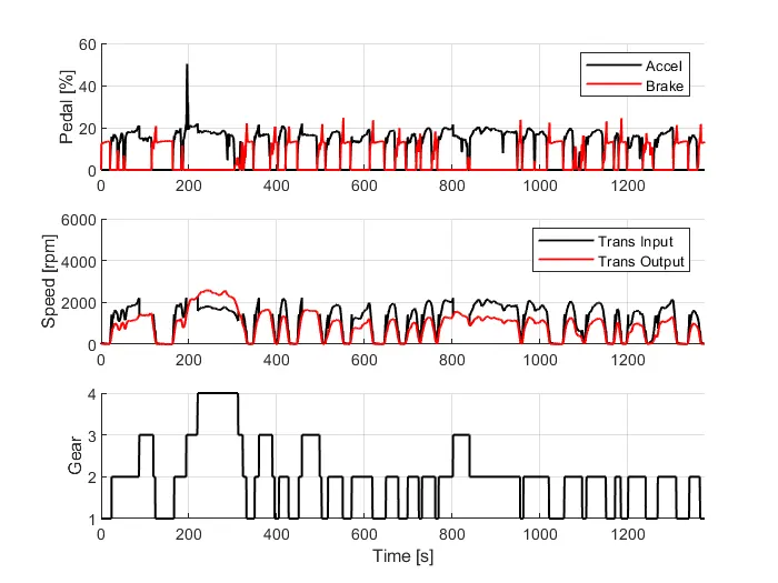
Accelerator and brake pedal, gear command, vehicle desired and actual speed, vehicle distance using subplots.

Engine Operating Points on Engine Fuel Map -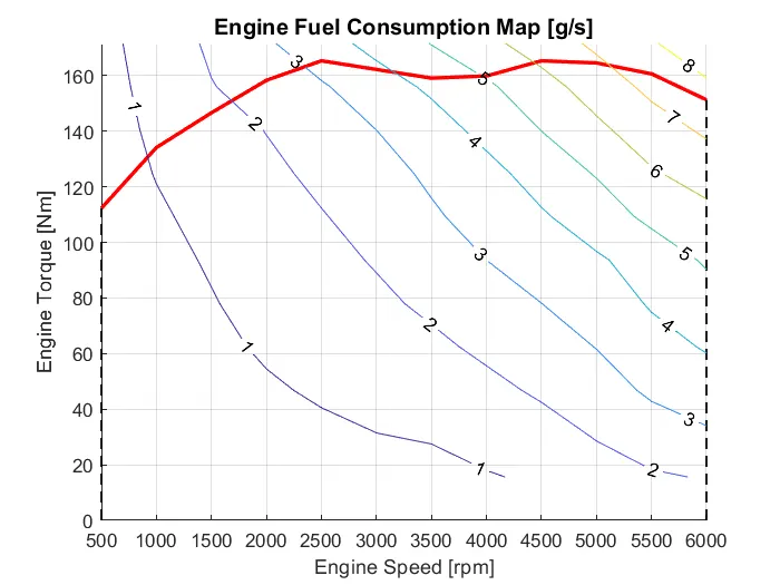

Fuel Consumption Vs Fuel Rate

Subplots between Engine Power , Engine Torque , Engine Fuel Consumption and Engine Fuel Rate

For HWFET Cycle -

Accelerator and brake pedal, gear command, vehicle desired and actual speed, vehicle distance using subplots.

Fuel Consumption Vs Fuel Rate

Engine Operating Points on Engine Fuel Map -

Subplots between Engine Power , Engine Torque , Engine Fuel Consumption and Engine Fuel Rate

Conclusion -

CONCLUSION

• Hence, the forward energy-based fuel consumption model of a conventional vehicle has been successfully Simulated using MATLAB and Simulink.
• Analyses and understands vehicle operating points based on engine speed, torque, transmission speed, pedal positions, gear, and distance travelled.
• Post process calculations were performed and the required graphs were successfully plotted.
• Successfully calculated vehicle fuel efficiency numbers (kmpl) for the given city cycle (UDDS) and highway cycle (HWFET)