Project 1

What is CAN?-CAN is short for ‘controller area network’. Controller area network is an electronic communication bus defined by the ISO 11898 standards. Those standards define how communication happens, how wiring is configured and how messages are constructed, among other things. To get deeper into the details of CAN, the CAN bus is a broadcast type of bus. This means that all nodes can “hear” all transmissions. There is no way to send a message to just a specific node; all nodes will invariably pick up all traffic. The CAN hardware, however, provides local filtering so that each node may react only on the interesting messages. We’ll discuss this more in Section 2, “CAN Messages”. In this system, the modules are connected to the bus in a wired-and fashion: if just one node is driving the bus to a logical 0, then the whole bus is in that state regardless of the number of nodes transmitting a logical 1.

The CAN standard defines four different message types. The messages uses a clever scheme of bit-wise arbitration to control access to the bus, and each message is tagged with a priority.

The CAN standard also defines an elaborate scheme for error handling and confinement which is described in more detail in Section 7, “CAN Error Handling”.

Bit timing and clock synchronization is discussed in Section 6 of this tutorial. Here’s a bit timing calculator you can use to calculate the CAN bus parameters and register settings.

CAN bus wiring may be implemented using different physical layers (Section 3), some of which are described here, and there are also a fair number of CAN bus connector types (Section 5) in use. We also provide a number of oscilloscope pictures (Section 4) for those interested in the details of a message.

CAN Messages

The CAN bus is a broadcast type of bus. This means that all nodes can ‘hear’ all transmissions. There is no way to send a message to just a specific node; all nodes will invariably pick up all traffic. The CAN hardware, however, provides local filtering so that each node may react only on the interesting messages.

The CAN messages

CAN uses short messages – the maximum utility load is 94 bits. There is no explicit address in the messages; instead, the messages can be said to be contents-addressed, that is, their contents implicitly determines their address.

Message Types

There are four different message types (or ‘frames’) on a CAN bus:

1.Data Frame

2. Remote Frame
3. Error Frame
4. Overload Frame

1.The Data Frame

Summary: “Hello everyone, here’s some data labeled X, hope you like it!”

The Data Frame is the most common message type. It comprises the following major parts (a few details are omitted for the sake of brevity): the Arbitration Field, which determines the priority of the message when two or more nodes are contending for the bus. The Arbitration Field contains:

For CAN 2.0A, an 11-bit Identifier and one bit, the RTR bit, which is dominant for data frames.

For CAN 2.0B, a 29-bit Identifier (which also contains two recessive bits: SRR and IDE) and the RTR bit.

the Data Field, which contains zero to eight bytes of data.

the CRC Field, which contains a 15-bit checksum calculated on most parts of the message. This checksum is used for error detection.

an Acknowledgement Slot; any CAN controller that has been able to correctly receive the message sends an Acknowledgement bit at the end of each message. The transmitter checks for the presence of the Acknowledge bit and retransmits the message if no acknowledge was detected.

Note 1: It is worth noting that the presence of an Acknowledgement Bit on the bus does not mean that any of the intended addressees has received the message. The only thing we know is that one or more nodes on the bus has received it correctly.

Note 2: The Identifier in the Arbitration Field is not, despite of its name, necessarily identifying the contents of the message.

A CAN 2.0A (“standard CAN”) Data Frame.

A CAN 2.0B (“extended CAN”) Data Frame.

The Remote Frame

Summary: “Hello everyone, can somebody please produce the data labeled X?”

The Remote Frame is just like the Data Frame, with two important differences: it is explicitly marked as a Remote Frame (the RTR bit in the Arbitration Field is recessive), and there is no Data Field. The intended purpose of the Remote Frame is to solicit the transmission of the corresponding Data Frame. If, say, node A transmits a Remote Frame with the Arbitration Field set to 234, then node B, if properly initialized, might respond with a Data Frame with the Arbitration Field also set to 234.

Remote Frames can be used to implement a request-response type of bus traffic management. In practice, however, the Remote Frame is little used. It is also worth noting that the CAN standard does not prescribe the behaviour outlined here. Most CAN controllers can be programmed either to automatically respond to a Remote Frame, or to notify the local CPU instead.

There’s one catch with the Remote Frame: the Data Length Code must be set to the length of the expected response message. Otherwise the arbitration will not work.

A Remote Frame (2.0A type)

Sometimes it is claimed that the node responding to the Remote Frame is starting its transmission as soon as the identifier is recognized, thereby “filling up” the empty Remote Frame. This is not the case.

The Error Frame

Summary: (everyone, aloud) “OH DEAR, LET’S TRY AGAIN”

Simply put, the Error Frame is a special message that violates the framing rules of a CAN message. It is transmitted when a node detects a fault and will cause all other nodes to detect a fault – so they will send Error Frames, too. The transmitter will then automatically try to retransmit the message. There is an elaborate scheme of error counters that ensures that a node can’t destroy the bus traffic by repeatedly transmitting Error Frames.

The Error Frame consists of an Error Flag, which is 6 bits of the same value (thus violating the bit-stuffing rule) and an Error Delimiter, which is 8 recessive bits. The Error Delimiter provides some space in which the other nodes on the bus can send their Error Flags when they detect the first Error Flag.

An Error Frame

The Overload Frame

Summary: “I’m a very busy little 82526, could you please wait for a moment?”

The Overload Frame is mentioned here just for completeness. It is very similar to the Error Frame regarding the format and it is transmitted by a node that becomes too busy. The Overload Frame is not used very often, as today’s CAN controllers are clever enough not to use it. In fact, the only controller that will generate Overload Frames is the now obsolete 82526.

Standard vs. Extended CAN

Originally, the CAN standard defined the length of the Identifier in the Arbitration Field to eleven (11) bits. Later, customer demand forced an extension of the standard. The new format is often called Extended CAN and allows no less than twenty-nine (29) bits in the Identifier. To differentiate between the two frame types, a reserved bit in the Control Field was used.

The standards are formally called

2.0A, with 11-bit Identifiers only,

2.0B, extended version with the full 29-bit Identifiers (or the 11-bit, you can mix them.) A 2.0B node can be

“2.0B active”, i.e. it can transmit and receive extended frames, or

“2.0B passive”, i.e. it will silently discard received extended frames (but see below.)

1.x refers to the original specification and its revisions.

New CAN controllers today are usually of the 2.0B type. A 1.x or 2.0A type controller will get very upset if it receives messages with 29 arbitration bits. A 2.0B passive type controller will tolerate them, acknowledge them if they are correct and then – discard them; a 2.0B active type controller can both transmit and receive them.

Controllers implementing 2.0B and 2.0A (and 1.x) are compatible – and may be used on the same bus – if the controllers implementing 2.0B refrain from sending extended frames!

Sometimes people advocate that standard CAN is “better” than Extended CAN because there is more overhead in the Extended CAN messages. This is not necessarily true. If you use the Arbitration Field for transmitting data, then Extended CAN may actually have a lower overhead than Standard CAN has.

Basic CAN vs. Full CAN

The terms “Basic CAN” and “Full CAN” originate from the childhood of CAN. Once upon a time there was the Intel 82526 CAN controller which provided a DPRAM-style interface to the programmer. Then came along Philips with the 82C200 which used a FIFO- (queue-) oriented programming model and limited filtering abilities. To distinguish between the two programming models, people for some reason termed the Intel way as “Full CAN” and the Philips way as “Basic CAN”. Today, most CAN controllers allow for both programming models, so there is no reason to use the terms “Full CAN” and “Basic CAN” – in fact, these terms can cause confusion and should be avoided.

Of course, a “Full CAN” controller can communicate with a “Basic CAN” controller and vice versa. There are no compatibility problems.

Bus Arbitration and Message Priority

The message arbitration (the process in which two or more CAN controllers agree on who is to use the bus) is of great importance for the actually available bandwidth for data transmission.

Any CAN controller may start a transmission when it has detected an idle bus. This may result in two or more controllers starting a message (almost) at the same time. The conflict is resolved in the following way. The transmitting nodes monitor the bus while they are sending. If a node detects a dominant level when it is sending a recessive level itself, it will immediately quit the arbitration process and become a receiver instead. The arbitration is performed over the whole Arbitration Field and when that field has been sent, exactly one transmitter is left on the bus. This node continues the transmission as if nothing had happened. The other potential transmitters will try to retransmit their messages when the bus becomes available next time. No time is lost in the arbitration process.

An important condition for this bit-wise arbitration to succeed is that no two nodes may transmit the same Arbitration Field. There is one exception to this rule: if the message contains no data, then any node may transmit that message.

Since the bus is wired-and and a Dominant bit is logically 0, it follows that the message with the numerically lowest Arbitration Field will win the arbitration.

Q: What happens if a node is alone on the bus and tries to transmit?

A: The node will, of course, win the arbitration and happily proceeds with the message transmission. But when the time comes for acknowledging… no node will send a dominant bit during the ACK slot, so the transmitter will sense an ACK error, send an error flag, increase its transmit error counter by 8 and start a retransmission. This will happen 16 times; then the transmitter will go error passive. By a special rule in the error confinement algorithm, the transmit error counter is not further increased if the node is error passive and the error is an ACK error. So the node will continue to transmit forever, at least until someone acknowledges the message.

Message Addressing and Identification

It is worth noting once again that there is no explicit address in the CAN messages. Each CAN controller will pick up all traffic on the bus, and using a combination of hardware filters and software, determine if the message is “interesting” or not.

In fact, there is no notion of message addresses in CAN. Instead, the contents of the messages is identified by an identifier which is present somewhere in the message. CAN messages are said to be “contents-addressed”.

A conventional message address would be used like “Here’s a message for node X”. A contents-addressed message is like “Here’s a message containing data labeled X”. The difference between these two concepts is small but significant.

The contents of the Arbitration Field is, per the Standard, used to determine the message’s priority on the bus. All CAN controllers will also use the whole (some will use just a part) of the Arbitration Field as a key in the hardware filtration process.

The Standard does not say that the Arbitration Field must be used as a message identifier. It’s nevertheless a very common usage.

A note on the Identifier Values

We said that 11 (CAN 2.0A) or 29 (CAN 2.0B) bits is available in the Identifier. This is not entirely correct. Due to compability with a certain old CAN controller (guess which?), identifiers must not have the 7 most significant bits set to all ones, so only the identifiers 0..2031 are left for the 11-bit identifiers, and the user of 29-bit identifiers can use 532676608 different values.

Note that all other CAN controllers accept the “illegal” identifiers, so in a modern CAN system identifiers 2032..2047 can be used without restrictions.

CAN Physical Layers

The CAN Bus

The CAN bus uses Non-Return To Zero (NRZ) with bit-stuffing. There are two different signaling states: dominant (logically 0) and recessive (logically 1). These correspond to certain electrical levels which depend on the physical layer used (there are several.) The modules are connected to the bus in a wired-and fashion: if just one node is driving the bus to the dominant state, then the whole bus is in that state regardless of the number of nodes transmitting a recessive state.

Different Physical Layers

A physical layer defines the electrical levels and signaling scheme on the bus, the cable impedance and similar things.

There are several different physical layers:

The most common type is the one defined by the CAN standard, part ISO 11898-2, and it’s a two-wire balanced signaling scheme. It is also sometimes known as “high-speed CAN”.

Another part of the same ISO standard, ISO 11898-3, defines another two-wire balanced signaling scheme for lower bus speeds. It is fault tolerant, so the signaling can continue even if one bus wire is cut or shorted to ground or Vbat. It is sometimes known as “low-speed CAN”.

SAE J2411 defines a single-wire (plus ground, of course) physical layer. It’s used chiefly in cars – e.g. GM-LAN.

Several proprietary physical layers do exist.

Modifications of RS485 were used in the Old Ages when CAN drivers didn’t exist.

Go to Page 6 to view a number of oscilloscope pictures for those interested in the details of a message.

Different physical layers can not, as a rule, interoperate. Some combinations may work, or seem to work, under good conditions. For example, using both “high-speed” and “low-speed” transceivers on the same bus can work … sometimes.

A great many CAN transceiver chips are manufactured by NXP; alternative vendors include Bosch, Infineon, Texas Instruments and Vishay Siliconix.

A very common type is the 82C250 transceiver which implements the physical layer defined by ISO 11898. The 82C251 is an improved version.

A common transceiver for “low-speed CAN” is TJA1054 from NXP.

Maximum Bus Speed

The maximum speed of a CAN bus, according to the standard, is 1 Mbit/second. Some CAN controllers will nevertheless handle higher speeds than 1Mbit/s and may be considered for special applications.

Low-speed CAN (ISO 11898-3, see above) can go up to 125 kbit/s.

Single-wire CAN can go up to around 50 kbit/s in its standard mode and, using a special high-speed mode used e.g. for ECU programming, up to around 100 kbit/s.

Minimum Bus Speed

Be aware that some bus transceivers will not allow you to go below a certain bit rate. For example, using 82C250 or 82C251 you can go down to 10 kbit/s without problems, but if you use the TJA1050 instead you can’t go below around 50 kbit/s. Check the data sheet.

Maximum Cable Length

At a speed of 1 Mbit/s, a maximum cable length of about 40 meters (130 ft.) can be used. This is because the arbitration scheme requires that the wave front of the signal be able to propagate to the most remote node and back again before the bit is sampled. In other words, the cable length is restricted by the speed of light. A proposal to increase the speed of light has been considered but was turned down because of its inter-galactic consequences.

Other maximum cable lengths are (these values are approximate):

100 meters (330 ft) at 500 kbit/s

200 meters (650 ft) at 250 kbit/s

500 meters (1600 ft) at 125 kbit/s

6 kilometers (20000 ft) at 10 kbit/s

If optocouplers are used to provide galvanic isolation, the maximum bus length is decreased accordingly. Hint: use fast optocouplers, and look at the delay through the device, not at the specified maximum bit rate.

Bus Termination

An ISO 11898 CAN bus must be terminated. This is done using a resistor of 120 Ohms in each end of the bus. The termination serves two purposes:

Remove the signal reflections at the end of the bus.

Ensure the bus gets correct DC levels.

An ISO 11898 CAN bus must always be terminated regardless of its speed. I’ll repeat this: an ISO 11898 CAN bus must always be terminated regardless of its speed. For laboratory work just one terminator might be enough. If your CAN bus works even though you haven’t put any terminators on it, you are just lucky.

Note that other physical layers, such as “low-speed CAN”, single-wire CAN, and others, may or may not require termination. But your vanilla high-speed ISO 11898 CAN bus will always require at least one terminator.

What Is a Log?

A log is perhaps the simplest possible storage abstraction. It is an append-only, totally ordered sequence of records ordered by time. It looks like this

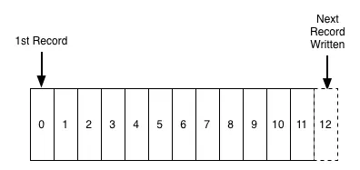
Records are appended to the end of the log and reads proceed left-to-right. Each entry is assigned a unique sequential log entry number.

The ordering of records defines a notion of "time" since entries to the left are defined to be older then entries to the right. The log entry number can be thought of as the "timestamp" of the entry. Describing this ordering as a notion of time seems a bit odd at first, but it has the convenient property that it is decoupled from any physical clock. This property will turn out to be essential as we get to distributed systems.

The contents and format of the records aren't important for the purposes of this discussion. Also, we can't just keep adding records to the log as we'll eventually run out of space. I'll come back to this in a bit.

So, a log is not all that different from a file or a table. A file is an array of bytes, a table is an array of records, and a log is just a kind of table or file where the records are sorted by time.

At this point you might be wondering why it is worth talking about something so simple? How is a append-only sequence of records in any way related to data systems? The answer is that logs have a specific purpose: they record what happened and when. For distributed data systems this is, in many ways, the very heart of the problem.

But before we get too far let me clarify something that is a bit confusing. Every programmer is familiar with another definition of logging—the unstructured error messages or trace info an application might write out to a local file using syslog or log4j. For clarity I will call this "application logging". The application log is a degenerative form of the log concept I am describing. The biggest difference is that text logs are meant to be primarily for humans to read and the "journal" or "data logs" I'm describing are built for programmatic access.

(Actually, if you think about it, the idea of humans reading through logs on individual machines is something of an anachronism. This approach quickly becomes an unmanageable strategy when many services and servers are involved and the purpose of logs quickly becomes as an input to queries and graphs to understand behavior across many machines—something for which english text in files is not nearly as appropriate as the kind structured log described here.)

Logs in databases

I don't know where the log concept originated—probably it is one of those things like binary search that is too simple for the inventor to realize it was an invention. It is present as early as IBM's System R. The usage in databases has to do with keeping in sync the variety of data structures and indexes in the presence of crashes. To make this atomic and durable, a database uses a log to write out information about the records they will be modifying, before applying the changes to all the various data structures it maintains. The log is the record of what happened, and each table or index is a projection of this history into some useful data structure or index. Since the log is immediately persisted it is used as the authoritative source in restoring all other persistent structures in the event of a crash.

Over-time the usage of the log grew from an implementation detail of ACID to a method for replicating data between databases. It turns out that the sequence of changes that happened on the database is exactly what is needed to keep a remote replica database in sync. Oracle, MySQL, and PostgreSQL include log shipping protocols to transmit portions of log to replica databases which act as slaves. Oracle has productized the log as a general data subscription mechanism for non-oracle data subscribers with their X-Streams and Golden Gate and similar facilities in MySQL and PostgreSQL are key components of many data architectures.

Because of this origin, the concept of a machine readable log has largely been confined to database internals. The use of logs as a mechanism for data subscription seems to have arisen almost by chance. But this very abstraction is ideal for supporting all kinds of messaging, data flow, and real-time data processing.

Logs in distributed systems

The two problems a log solves—ordering changes and distributing data—are even more important in distributed data systems. Agreeing upon an ordering for updates (or agreeing to disagree and coping with the side-effects) are among the core design problems for these systems.

The log-centric approach to distributed systems arises from a simple observation that I will call the State Machine Replication Principle:

If two identical, deterministic processes begin in the same state and get the same inputs in the same order, they will produce the same output and end in the same state.

This may seem a bit obtuse, so let's dive in and understand what it means.

Deterministic means that the processing isn't timing dependent and doesn't let any other "out of band" input influence its results. For example a program whose output is influenced by the particular order of execution of threads or by a call to get time of day or some other non-repeatable thing is generally best considered as non-deterministic.

The state of the process is whatever data remains on the machine, either in memory or on disk, at the end of the processing.

The bit about getting the same input in the same order should ring a bell—that is where the log comes in. This is a very intuitive notion: if you feed two deterministic pieces of code the same input log, they will produce the same output.

The application to distributed computing is pretty obvious. You can reduce the problem of making multiple machines all do the same thing to the problem of implementing a distributed consistent log to feed these processes input. The purpose of the log here is to squeeze all the non-determinism out of the input stream to ensure that each replica processing this input stays in sync.

When you understand it, there is nothing complicated or deep about this principle: it more or less amounts to saying "deterministic processing is deterministic". Nonetheless, I think it is one of the more general tools for distributed systems design.

One of the beautiful things about this approach is that the time stamps that index the log now act as the clock for the state of the replicas—you can describe each replica by a single number, the timestamp for the maximum log entry it has processed. This timestamp combined with the log uniquely captures the entire state of the replica.

There are a multitude of ways of applying this principle in systems depending on what is put in the log. For example, we can log the incoming requests to a service, or the state changes the service undergoes in response to request, or the transformation commands it executes. Theoretically, we could even log a series of machine instructions for each replica to execute or the method name and arguments to invoke on each replica. As long as two processes process these inputs in the same way, the processes will remaining consistent across replicas.

Different groups of people seem to describe the uses of logs differently. Database people generally differentiate between physical and logical logging. Physical logging means logging the contents of each row that is changed. Logical logging means logging not the changed rows but the SQL commands that lead to the row changes (the insert, update, and delete statements).

The distributed systems literature commonly distinguishes two broad approaches to processing and replication. The "state machine model" usually refers to an active-active model where we keep a log of the incoming requests and each replica processes each request. A slight modification of this, called the "primary-backup model", is to elect one replica as the leader and allow this leader to process requests in the order they arrive and log out the changes to its state from processing the requests. The other replicas apply in order the state changes the leader makes so that they will be in sync and ready to take over as leader should the leader fail.

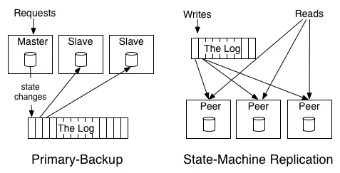
To understand the difference between these two approaches, let's look at a toy problem. Consider a replicated "arithmetic service" which maintains a single number as its state (initialized to zero) and applies additions and multiplications to this value. The active-active approach might log out the transformations to apply, say "+1", "*2", etc. Each replica would apply these transformations and hence go through the same set of values. The "active-passive" approach would have a single master execute the transformations and log out the result, say "1", "3", "6", etc. This example also makes it clear why ordering is key for ensuring consistency between replicas: reordering an addition and multiplication will yield a different result. The distributed log can be seen as the data structure which models the problem of consensus. A log, after all, represents a series of decisions on the "next" value to append. You have to squint a little to see a log in the Paxos family of algorithms, though log-building is their most common practical application. With Paxos, this is usually done using an extension of the protocol called "multi-paxos", which models the log as a series of consensus problems, one for each slot in the log. The log is much more prominent in other protocols such as ZAB, RAFT, and View stamped Replication, which directly model the problem of maintaining a distributed, consistent log.

My suspicion is that our view of this is a little bit biased by the path of history, perhaps due to the few decades in which the theory of distributed computing outpaced its practical application. The consensus problem is a bit too simple. Computer systems rarely need to decide a single value, they almost always handle a sequence of requests. So, a log, rather than a simple single-value register, is the more natural abstraction.

Furthermore, the focus on the algorithms obscures the underlying log abstraction systems need. I suspect we will end up focusing more on the log as a commoditized building block irrespective of its implementation in the same way we often talk about a hash table without bothering to get in the details of whether we mean the murmur hash with linear probing or some other variant. The log will become something of a commoditized interface, with many algorithms and implementations competing to provide the best guarantees and optimal performance.

Changelog 101: Tables and Events are Dual

Let's come back to databases for a bit. There is a fascinating duality between a log of changes and a table. The log is like the list of all credits and debits and bank processes; a table is all the current account balances. If you have a log of changes, you can apply these changes to create the table capturing the current state. This table will record the latest state for each key (as of a particular log time). There is a sense in which the log is the more fundamental data structure: in addition to creating the original table you can also transform it to create all kinds of derived tables. (And yes, table can mean keyed data store for the non-relational folks.)

This process works in reverse too: if you have a table taking updates, you can record these changes and publish a "changelog" of all the updates to the state of the table. This changelog is exactly what you need to support near-real-time replicas. So in this sense you can see tables and events as dual: tables support data at rest and logs capture change. The magic of the log is that if it is a complete log of changes, it holds not only the contents of the final version of the table, but also allows recreating all other versions that might have existed. It is, effectively, a sort of backup of every previous state of the table.

This might remind you of source code version control. There is a close relationship between source control and databases. Version control solves a very similar problem to what distributed data systems must solve—managing distributed, concurrent changes in state. A version control system usually models the sequence of patches, which is in effect a log. You interact directly with a checked out "snapshot" of the current code which is analogous to the table. You will note that in version control systems, as in other distributed stateful systems, replication happens via the log: when you update, you pull down just the patches and apply them to your current snapshot.

Some people have seen some of these ideas recently from Diatomic, a company selling a log-centric database. This presentation gives a great overview of how they have applied the idea in their system. These ideas are not unique to this system, of course, as they have been a part of the distributed systems and database literature for well over a decade.

This may all seem a little theoretical. Do not despair! We'll get to practical stuff quickly.

What's next

In the remainder of this article, I will try to give a flavours of what a log is good for that goes beyond the internals of distributed computing or abstract distributed computing models. This includes:

Data Integration—Making all of an organization's data easily available in all its storage and processing systems.

Real-time data processing—Computing derived data streams.

Distributed system design—How practical systems can by simplified with a log-centric design.

These uses all resolve around the idea of a log as a stand-alone service.

In each case, the usefulness of the log comes from simple function that the log provides: producing a persistent, re-playable record of history. Surprisingly, at the core of these problems is the ability to have many machines playback history at their own rate in a deterministic manner.

Part Two: Data Integration

Let me first say what I mean by "data integration" and why I think it's important, then we'll see how it relates back to logs.

Data integration is making all the data an organization has available in all its services and systems.

This phrase "data integration" isn't all that common, but I don't know a better one. The more recognizable term ETL usually covers only a limited part of data integration—populating a relational data warehouse. But much of what I am describing can be thought of as ETL generalized to cover real-time systems and processing flows.

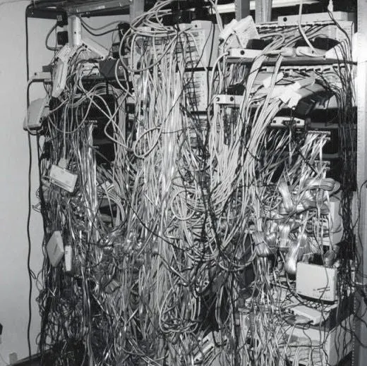
You don't hear much about data integration in all the breathless interest and hype around the idea of big data, but nonetheless, I believe this mundane problem of "making the data available" is one of the more valuable things an organization can focus on.

Effective use of data follows a kind of Maslow's hierarchy of needs. The base of the pyramid involves capturing all the relevant data, being able to put it together in an applicable processing environment (be that a fancy real-time query system or just text files and python scripts). This data needs to be modelled in a uniform way to make it easy to read and process. Once these basic needs of capturing data in a uniform way are taken care of it is reasonable to work on infrastructure to process this data in various ways—MapReduce, real-time query systems, etc.

It's worth noting the obvious: without a reliable and complete data flow, a Hadoop cluster is little more than a very expensive and difficult to assemble space heater. Once data and processing are available, one can move concern on to more refined problems of good data models and consistent well understood semantics. Finally, concentration can shift to more sophisticated processing—better visualization, reporting, and algorithmic processing and prediction.

In my experience, most organizations have huge holes in the base of this pyramid—they lack reliable complete data flow—but want to jump directly to advanced data modelling techniques. This is completely backwards.

So the question is, how can we build reliable data flow throughout all the data systems in an organization?

Data Integration: Two complications

Two trends make data integration harder.

The event data firehose

The first trend is the rise of event data. Event data records things that happen rather than things that are. In web systems, this means user activity logging, but also the machine-level events and statistics required to reliably operate and monitor a data centre’s worth of machines. People tend to call this "log data" since it is often written to application logs, but that confuses form with function. This data is at the heart of the modern web: Google's fortune, after all, is generated by a relevance pipeline built on clicks and impressions—that is, events.

And this stuff isn't limited to web companies, it's just that web companies are already fully digital, so they are easier to instrument. Financial data has long been event centric. RFID adds this kind of tracking to physical objects. I think this trend will continue with the digitization of traditional businesses and activities.

This type of event data records what happened and tends to be several orders of magnitude larger than traditional database uses. This presents significant challenges for processing.

The explosion of specialized data systems

The second trend comes from the explosion of specialized data systems that have become popular and often freely available in the last five years. Specialized systems exist for OLAP, search, simple online storage, batch processing, graph analysis, and so on.

The combination of more data of more varieties and a desire to get this data into more systems leads to a huge data integration problem.

Log-structured data flow

The log is the natural data structure for handling data flow between systems. The recipe is very simple:

Take all the organization's data and put it into a central log for real-time subscription.

Each logical data source can be modelled as its own log. A data source could be an application that logs out events (say clicks or page views), or a database table that accepts modifications. Each subscribing system reads from this log as quickly as it can, applies each new record to its own store, and advances its position in the log. Subscribers could be any kind of data system—a cache, Hadoop, another database in another site, a search system, etc.

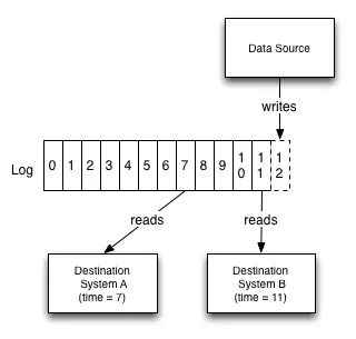
For example, the log concept gives a logical clock for each change against which all subscribers can be measured. This makes reasoning about the state of the different subscriber systems with respect to one another far simpler, as each has a "point in time" they have read up to.

To make this more concrete, consider a simple case where there is a database and a collection of caching servers. The log provides a way to synchronize the updates to all these systems and reason about the point of time of each of these systems. Let's say we write a record with log entry X and then need to do a read from the cache. If we want to guarantee we don't see stale data, we just need to ensure we don't read from any cache which has not replicated up to X.

The log also acts as a buffer that makes data production asynchronous from data consumption. This is important for a lot of reasons, but particularly when there are multiple subscribers that may consume at different rates. This means a subscribing system can crash or go down for maintenance and catch up when it comes back: the subscriber consumes at a pace it controls. A batch system such as Hadoop or a data warehouse may consume only hourly or daily, whereas a real-time query system may need to be up-to-the-second. Neither the originating data source nor the log has knowledge of the various data destination systems, so consumer systems can be added and removed with no change in the pipeline.