Project 1

3)

%%%%%%%%%%%%%%%%%%%%%%%%%%%%%%%%%%%%%%%%%%%%%%%%%%%%%%%%%%%%%%%%%%%%%

%% Skill-Lync -> Hybrid Drives Development

% Project 1 - Conventional Vehicle Model

% By - Ullekh Gambhira

% Description:

%% Initialization File

% Initialization file for loading the variables for the Conventional vehicle simulation model

%% Vehicle Parameters

M = 1500; % Vehicle weight [kg]

Cr = 0.015; % Rolling resistance coefficient

Rw = 0.35; % Rolling radius [m]

Cd = 0.33; % Drag coefficient

Af = 2; % Frontal area [m2]

rhoa = 1.225; % Air density [kg/m3]

Vwind = 0; % Wind velocity [kmph]

g = 9.81; % Gravitational acceleration [m/s2]

theta = 0; % Slope [deg]

myu_road_tire = 1; % Coefficient of friction between tire - road interface

%% Powertrain Parameters

FDR = 3.73; % Final Drive Ratio / Diff Ratio

DiffEff = 0.99; % Differential efficiency (assumed independent of operating conditions)

NumGear = 4; % Number of gears in transmission

TransGear = [1:NumGear]; % Transmission Gears

TransRatio = [3.06, 1.62, 1, 0.7]; % Corresponding Transmission ratios

TransEff = 0.90; % Transmission efficiency (assumed independent of operating conditions)

TC_SR = [0, .5, .6, .7, .8, .87, .92, .94, .96, .97, 1]; % Torque Converter Speed Ratio (Matlab default) -> TurbSpd/PumpSpd

TC_TR = [2.232, 1.5462, 1.4058, 1.2746, 1.1528, 1.0732, 1.0192, 1, 1, 1, 1]; % Torque Converter Torque Ratio (Matlab default) -> TurbTrq/PumpTrq

TC_Cf = 1e-4 * [.72558, .66322, .63463, .59042, .51331, .4144, .29287, .22444, .12186, .04386, 0]; % Torque Converter Capacity Factor (Matlab default) -> PumpTrq/PumpSpd^2 [Nm/rpm^2]

load Vehicle_Data/Engine_data_1_9L_Saturn_95kW

load Vehicle_Data/Trans_Shift_map

%% Driver Parameters

Kp = 10; % P gain for driver PI model

Ki = 1; % I gain for driver PI model

Drive_Cycle_Select = 1; % Drive cycle selection

% Drive cycle values in m/s

if Drive_Cycle_Select == 1

load DriveCycles/UDDS;

elseif Drive_Cycle_Select == 2

load DriveCycles/HWFET;

elseif Drive_Cycle_Select == 3

load DriveCycles/FTP;

elseif Drive_Cycle_Select == 4

load DriveCycles/US06;

elseif Drive_Cycle_Select == 5

load DriveCycles/NEDC;

elseif Drive_Cycle_Select == 6

load DriveCycles/WLTP;

end

time_end = cyc_time(end);

vel_end = cyc_vel(end);

--------------------------------------------------------------------------------------------------------------------------------------------

%%%%%%%%%%%%%%%%%%%%%%%%%%%%%%%%%%%%%%%%%%%%%%%%%%%%%%%%%%%%%%%%%%%%%

%% Skill-Lync -> Hybrid Drives Development

% Project 1 - Conventional Vehicle Model

% By - Ullekh Gambhira

% Description:

% The following file is to used with the Initialization file and Simulink

% results for post-processing of the data.

% The file is incomplete, has some examples of how the data is imported

% into a readable format, data analysis and plotting examples.

% Based on the project task, use commands in a similar format as given

% below, to analyse the data and generate required plots.

% You can change variable names if desired

%% Post-Processing File

% File for post-processing the Conventional vehicle simulation model data

%% Renaming variables

Time = out.tout;

Acc_Pdl = out.Acc_Pdl; % Accelerator pedal [%]

Brk_Pdl = out.Brk_Pdl; % Brake pedal [%]

Gear_Cmd = out.Gear_Cmd; % Transmission gear

Trans_In_Spd = out.Trans_In_Spd*30/pi; % Transmission input speed [rpm]

Trans_Out_Spd = out.Trans_Out_Spd*30/pi;% Transmission output speed [rpm]

Eng_Trq = out.Eng_Trq; % Engine brake torque [Nm]

Eng_Spd = out.Eng_Spd*30/pi; % Engine speed [rpm]

Eng_Fuel_Rate=out.Eng_Fuel_Rate;% Engine Fuel rate [gKW]

Eng_Fuel_Consump = out.Eng_Fuel_Consumption; % Engine fuel consumption [g]

Veh_Dist = out.Veh_Dist/1000; % Distance traveled by vehicle [km]

Veh_Spd = out.Veh_Spd*18/5; % Vehicle speed [kmph]

Wheel_Spd=out.Wheel_Spd*(30/pi);% Wheel speed [rpm]

Veh_Desired_Spd=out.Veh_Desired_Spd;% Vehicle Desired speed [kmph]

%% Data Analysis

Eng_Pwr = Eng_Spd*pi/30*Eng_Trq/1000; % Engine brake power [kW]

rho_petrol = 0.7197; % Density of petrol [kg/L]

kmpl = Veh_Dist(end)/(Eng_Fuel_Consump(end)/1000/rho_petrol); % Fuel economy [kmpl]

%% Plot the time trace for engine, transmission input, transmission output and wheel speed on one plot.

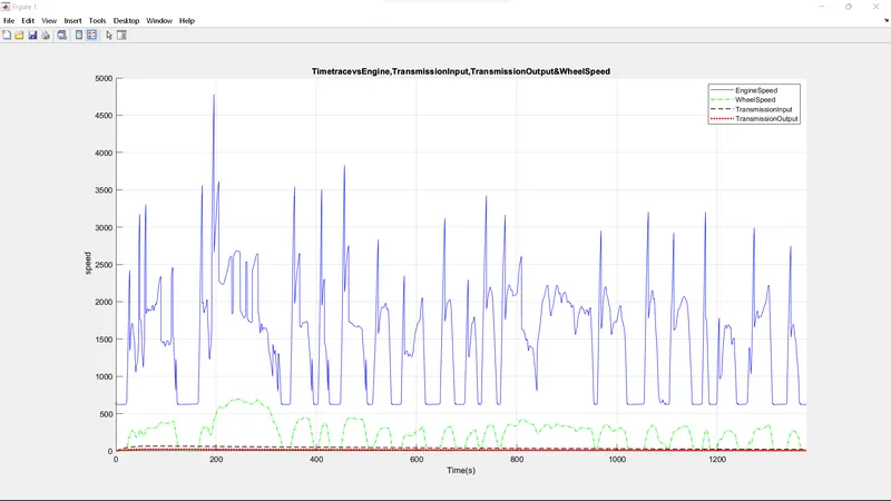
figure(1)

hold on;grid on;

title("TimetracevsEngine,TransmissionInput,TransmissionOutput&WheelSpeed")

plot(Eng_Spd,'b-');

plot(Wheel_Spd,'g-.','LineWidth',1);

plot(Trans_In_Spd,'k--','LineWidth',1);

plot(Trans_Out_Spd,'r:','LineWidth',2);xlabel("Time(s)");ylabel(" speed");

xlim([0,Time(end)]);

legend('EngineSpeed','WheelSpeed','TransmissionInput','TransmissionOutput');

%% Plot engine torque, engine power, fuel rate and fuel consumption using subplots.

figure(2)

xlabel('Time(s)');

%engine torque

subplot(4,1,1)

hold on;grid on;

plot(Eng_Trq,'k-','LineWidth',1);

ylabel("Engine Torque (Nm)");

xlim([0,Time(end)]);

%engine power

subplot(4,1,2)

hold on;grid on;

plot(Eng_Pwr,'k-','LineWidth',1);

ylabel("Engine Power (KW)");

xlim([0,Time(end)]);

%fuel rate

subplot(4,1,3)

hold on;grid on;

plot(Eng_Fuel_Rate,'k-','LineWidth',1);

ylabel("Engine Fuel rate");

xlim([0,Time(end)]);

%fuel consumption

subplot(4,1,4)

hold on;grid on;

plot(Eng_Fuel_Consump,'k-','LineWidth',1);

ylabel("Engine fuel concuption");

xlim([0,Time(end)]);

%% Plot accelerator and brake pedal, gear command,

% vehicle desired and actual speed, vehicle distance using subplots.

figure(3)

xlabel('Time(s)');

% Accelerator and brake pedal

subplot(4,1,1)

hold on;grid on;

plot(Acc_Pdl,'k-','LineWidth',1);

plot(Brk_Pdl,'r--','LineWidth',1);

xlim([0,Time(end)]);

legend('Acceleration pedal','Brake pedal');

% Gear command

subplot(4,1,2)

hold on;grid on;

plot(Gear_Cmd,'k-','LineWidth',1);

xlim([0,Time(end)]);

legend('Gear command');

% Vehicle desired and actual speed

subplot(4,1,3)

hold on;grid on;

plot(Veh_Spd,'k-','LineWidth',1);

plot(Veh_Desired_Spd,'r--','LineWidth',1);

xlim([0,Time(end)]);

legend('Actual speed','Desired speed');

% Vehicle distance

subplot(4,1,4)

hold on;grid on;

plot(Veh_Dist,'k-','LineWidth',1);

xlim([0,Time(end)]);

legend('Vehicle distance');

%% Plotting engine operating points on engine fuel map

figure('Name','Engine Operating Points');

hold on

grid on

title('Engine Operating Points','fontsize',12);

p1=plot(Eng_map_spd*30/pi,Eng_max_trq,'linewidth',2,'color','r');

p2=line([Eng_map_spd(end)*30/pi Eng_map_spd(end)*30/pi],[0 Eng_max_trq(end)]);

set(p2,'linewidth',2,'linestyle','--','color','g');

p3=line([Eng_map_spd(1)*30/pi Eng_map_spd(1)*30/pi],[0 Eng_max_trq(1)]);

set(p3,'linewidth',2,'linestyle','--','color','b');

[c,h] = contour(Eng_map_spd'*30/pi,Eng_map_trq,Eng_fuel_map');

clabel(c,h);

xlabel('Engine Speed [rpm]');

ylabel('Engine Torque [Nm]');

title('Engine Fuel Consumption Map [g/s]');

legend([p1 p3],{'Max Curve','Operating Points'});

axis([Eng_map_spd(1)*30/pi Eng_map_spd(end)*30/pi 0 Eng_map_trq(end)]);

--------------------------------------------------------------------------------------------------------------------------------------------

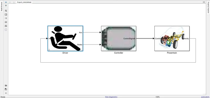
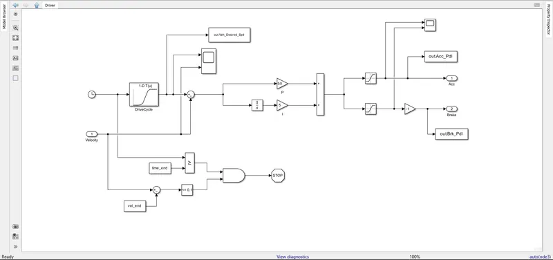
Driver subsystem:

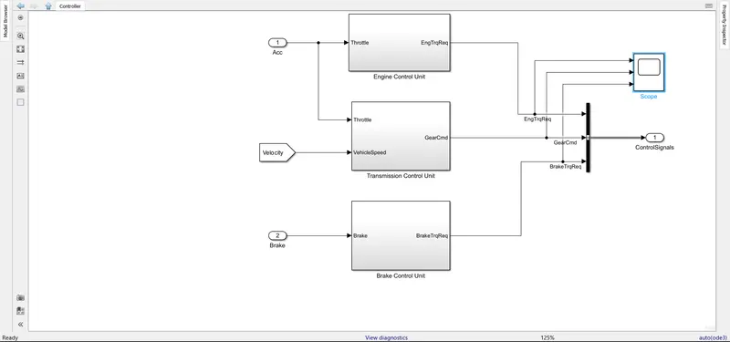
Controller subsystem:

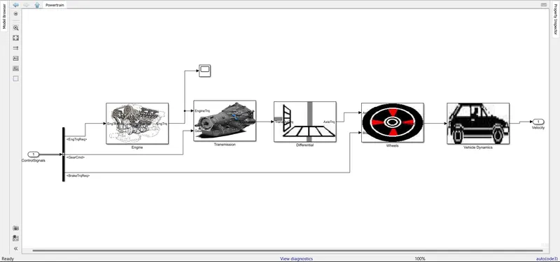
Powertrain subsystem:

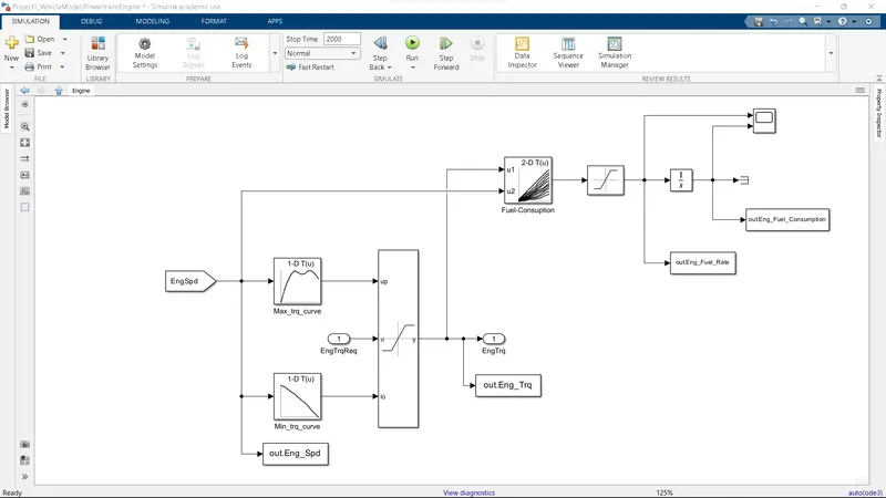
Engine subsystem

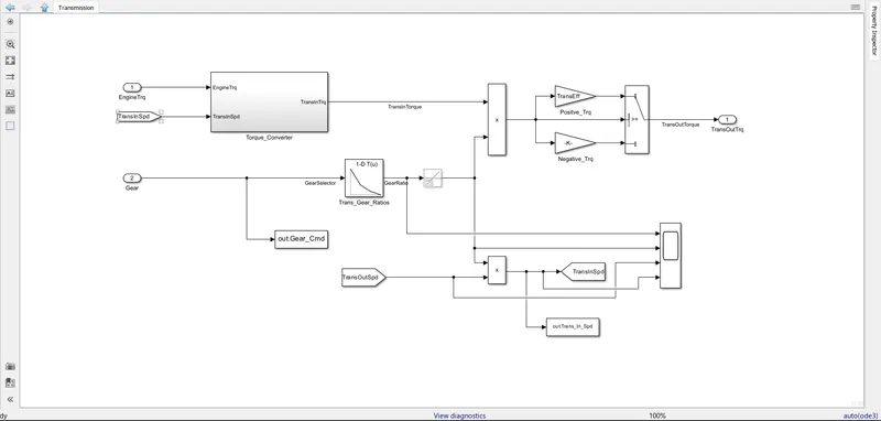
Transmission subsystem

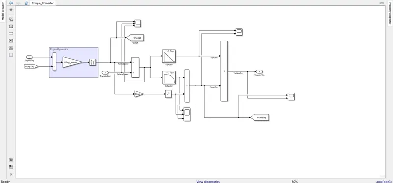
Torque converter

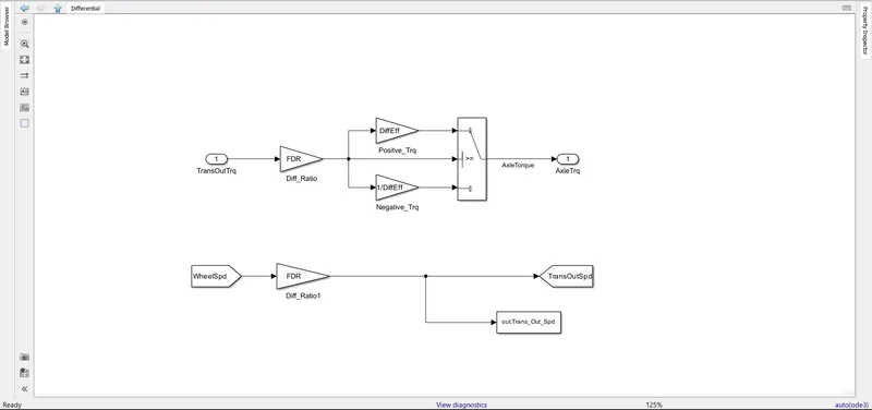
Differential

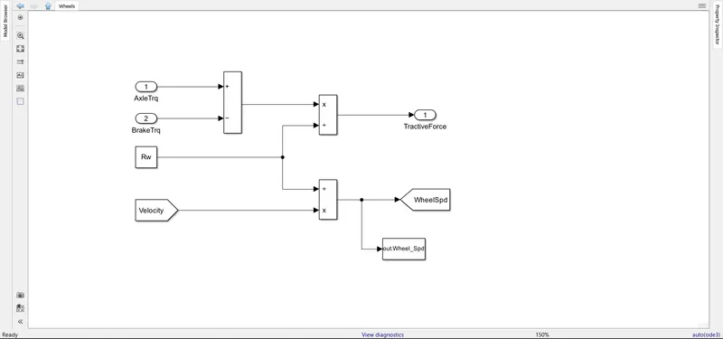
Wheel

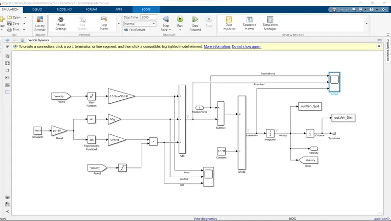
Vehicle dynamics subsystem

a)if Drive_Cycle_Select == 1: UDDS

--------------------------------------------------------------------------------------------------------------------------------------------

The graphes generated by the drive cycles shows their property.

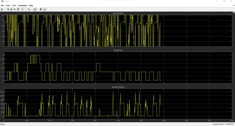
UDDS: Urban dynamometer driving schedule which represents city/urban driving conditions in which the vehicle is started cold and driven in stop-and-go traffic.

So, the stop and go traffic will cause the engine to rotate in higher and lower speed , which causes the flutuation seen in the figure1 plot. the transmisiion input and out speed controlles and maintain a constand speed is the reason for the control in the wheel speed.

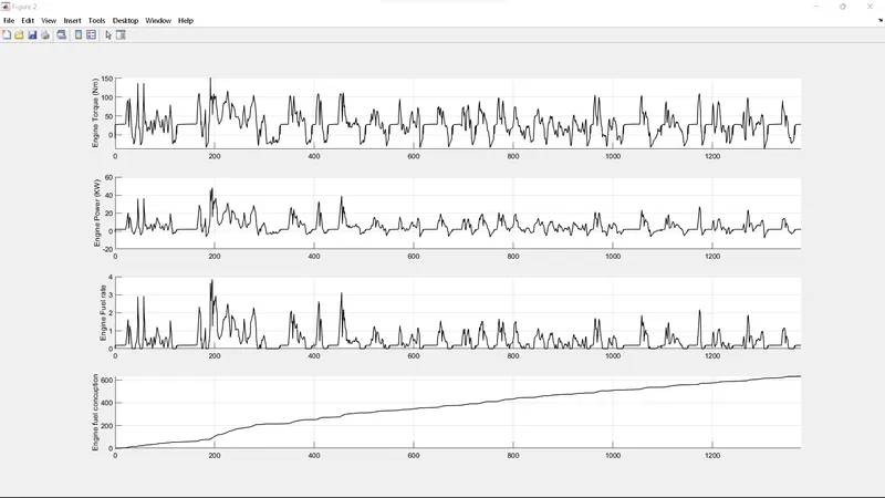
This stop and go condition will affect the perforance of the engine also in the similar way.

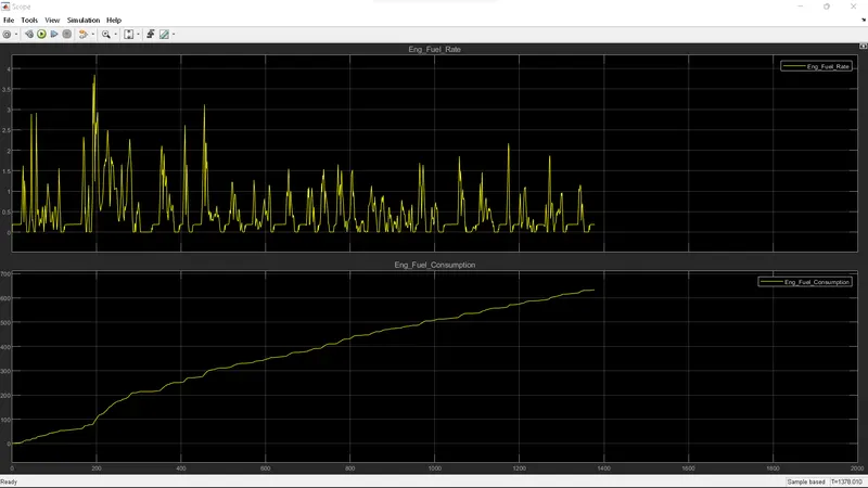
According to that, the engine torque and power out will also flatuate. Which will cause a increase in fuel consuption and affect engine fuel ratio accordingly which can be observed inthe figure 2 plot.

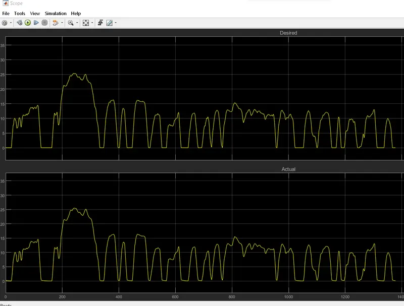
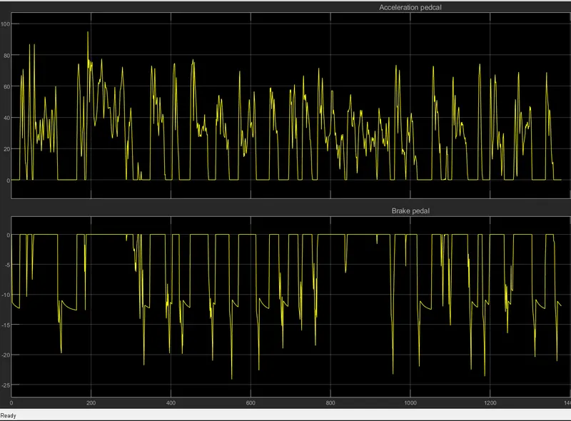
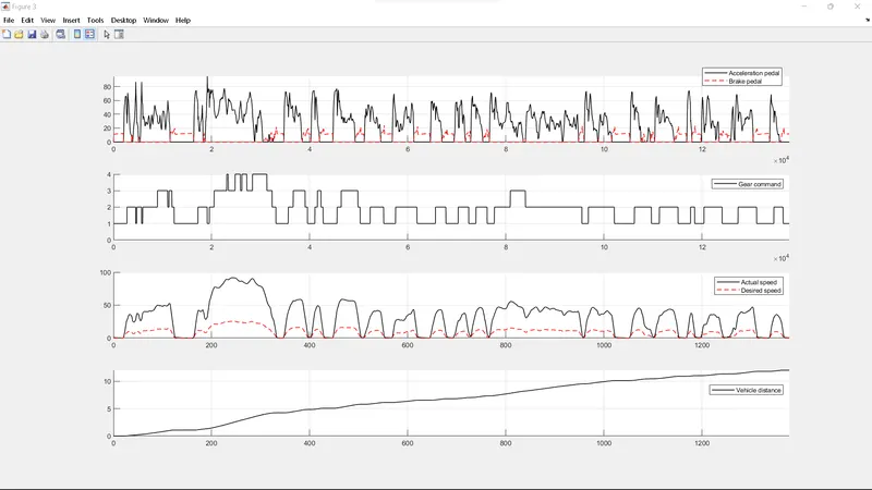
For the stop and go condition the accelerater and brake pedal is frequently engaged. and for the required speed the gear ration is also adujusted, and acceleration increase the gear no increases. So the actual speed is greater than the desired speed.

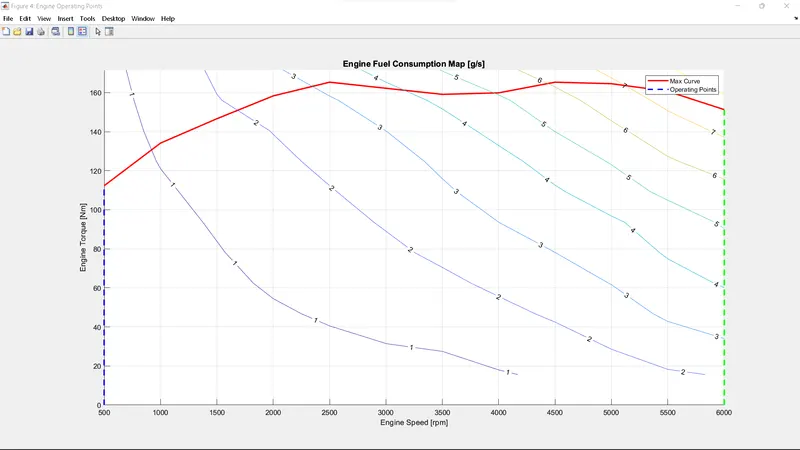
As the speed increases the engine torque increases which increases the fuel consumption which we can see in the figure 4 plot.

a)if Drive_Cycle_Select == 2: HWFET

Highway fuel economy driving schedule which represents a blend of rural and interstate highway driving with a warmup engine, as seen on longer trips in light traffic.

And those features are the reason for less flatualting engine and wheel speed.

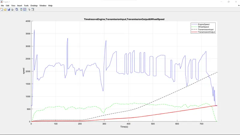
And because of the free flow of vehcile is the reason for less usage of brake pedal more frequent use of acceleratrion pedal. and gear will be also maitain for a longer period in higher number than UDDS.

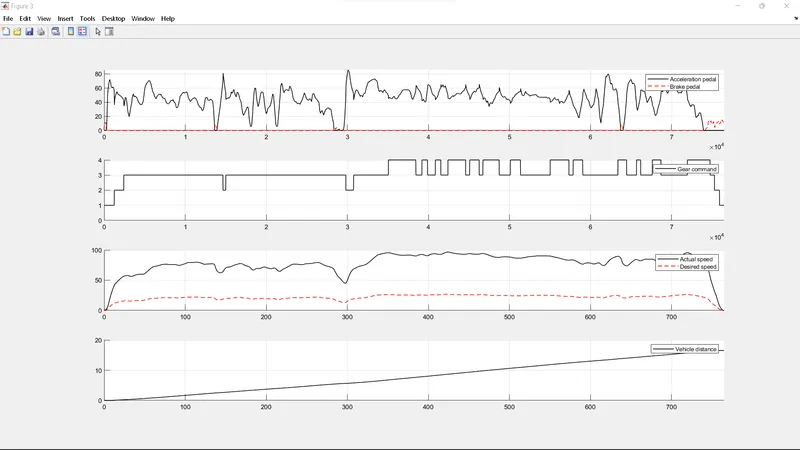
As the speed increases, so does the engine torque, which increases fuel consumption, as shown in the figure 4 plot.