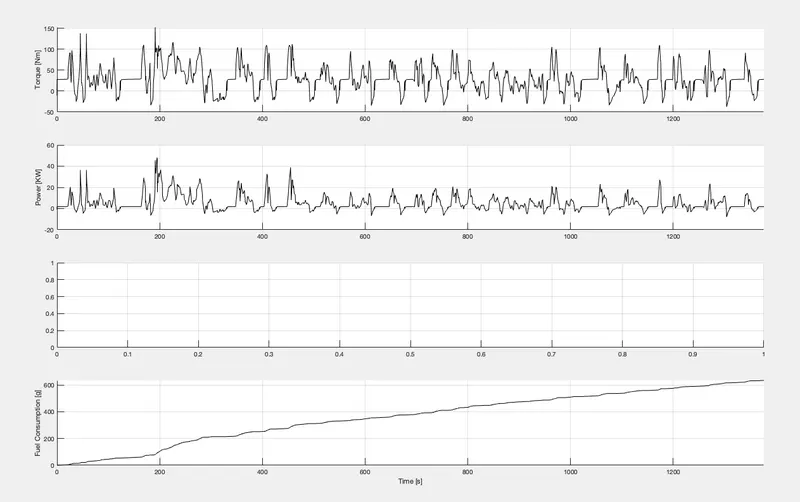
Project 1
INITIAL FILE:-
%%%%%%%%%%%%%%%%%%%%%%%%%%%%%%%%%%%%%%%%%%%%%%%%%%%%%%%%%%%%%%%%%%%%%
%% Skill-Lync -> Hybrid Drives Development
% Project 1 - Conventional Vehicle Model
% By - Ullekh Gambhira
% Description:
%% Initialization File
% Initialization file for loading the variables for the Conventional vehicle simulation model
%% Vehicle Parameters
M = 1500; % Vehicle weight [kg]
Cr = 0.015; % Rolling resistance coefficient
Rw = 0.35; % Rolling radius [m]
Cd = 0.33; % Drag coefficient
Af = 2; % Frontal area [m2]
rhoa = 1.225; % Air density [kg/m3]
Vwind = 0; % Wind velocity [kmph]
g = 9.81; % Gravitational acceleration [m/s2]
theta = 0; % Slope [deg]
myu_road_tire = 1; % Coefficient of friction between tire - road interface
%% Powertrain Parameters
FDR = 3.73; % Final Drive Ratio / Diff Ratio
DiffEff = 0.99; % Differential efficiency (assumed independent of operating conditions)
NumGear = 4; % Number of gears in transmission
TransGear = [1:NumGear]; % Transmission Gears
TransRatio = [3.06, 1.62, 1, 0.7]; % Corresponding Transmission ratios
TransEff = 0.90; % Transmission efficiency (assumed independent of operating conditions)
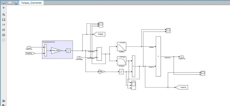
TC_SR = [0, .5, .6, .7, .8, .87, .92, .94, .96, .97, 1]; % Torque Converter Speed Ratio (Matlab default) -> TurbSpd/PumpSpd
TC_TR = [2.232, 1.5462, 1.4058, 1.2746, 1.1528, 1.0732, 1.0192, 1, 1, 1, 1]; % Torque Converter Torque Ratio (Matlab default) -> TurbTrq/PumpTrq
TC_Cf = 1e-4 * [.72558, .66322, .63463, .59042, .51331, .4144, .29287, .22444, .12186, .04386, 0]; % Torque Converter Capacity Factor (Matlab default) -> PumpTrq/PumpSpd^2 [Nm/rpm^2]
load Vehicle_Data/Engine_data_1_9L_Saturn_95kW
load Vehicle_Data/Trans_Shift_map
%% Driver Parameters
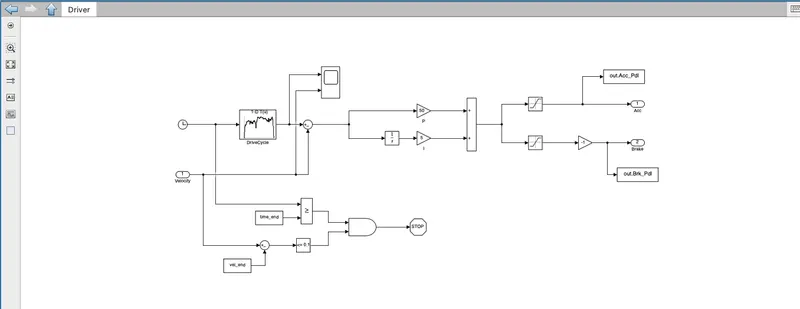
Kp = 10; % P gain for driver PI model
Ki = 1; % I gain for driver PI model
Drive_Cycle_Select = 1; % Drive cycle selection
% Drive cycle values in m/s
if Drive_Cycle_Select == 1
load DriveCycles/UDDS;
elseif Drive_Cycle_Select == 2
load DriveCycles/HWFET;
elseif Drive_Cycle_Select == 3
load DriveCycles/FTP;
elseif Drive_Cycle_Select == 4
load DriveCycles/US06;
elseif Drive_Cycle_Select == 5
load DriveCycles/NEDC;
elseif Drive_Cycle_Select == 6
load DriveCycles/WLTP;
end
time_end = cyc_time(end);
vel_end = cyc_vel(end);
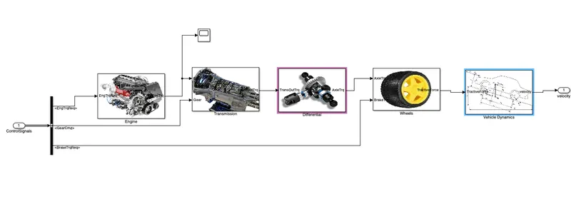
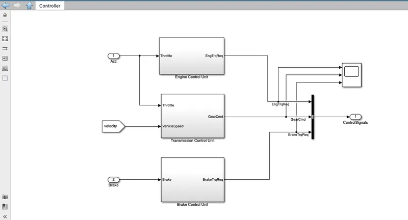
The below image is the major parts of vehicle this parts having number of sub parts and control systemes and driving systemes
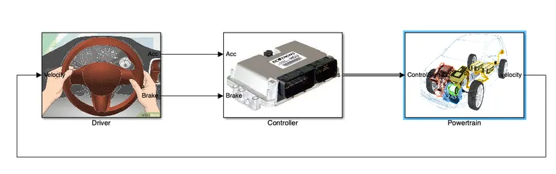
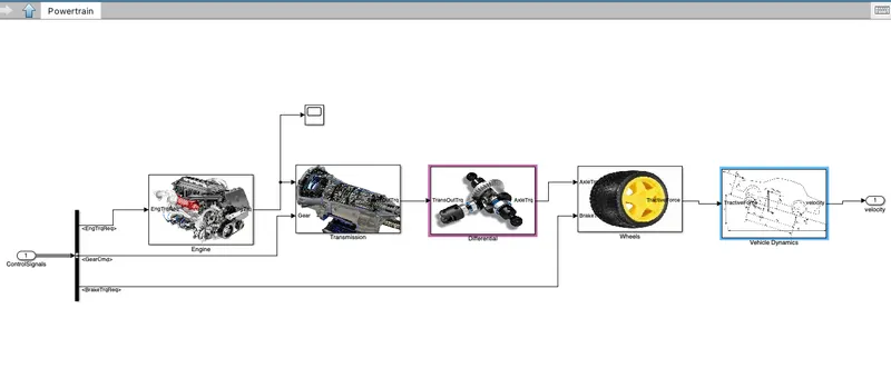
The Above powertrain block Having number of sub partes.each part having its own features and specificationes.
engine block is used to converting chemical energy to heat energy and heat to prusser ,pressur to mechanical energy converter.
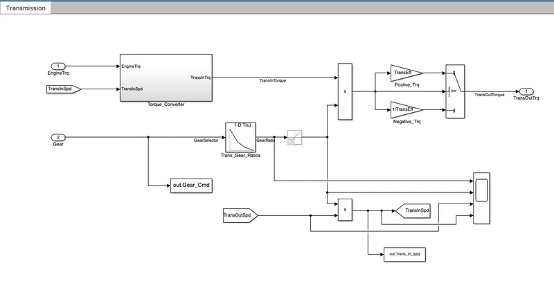
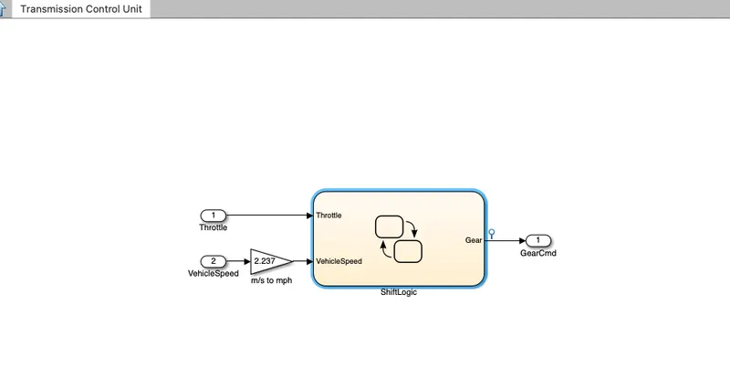
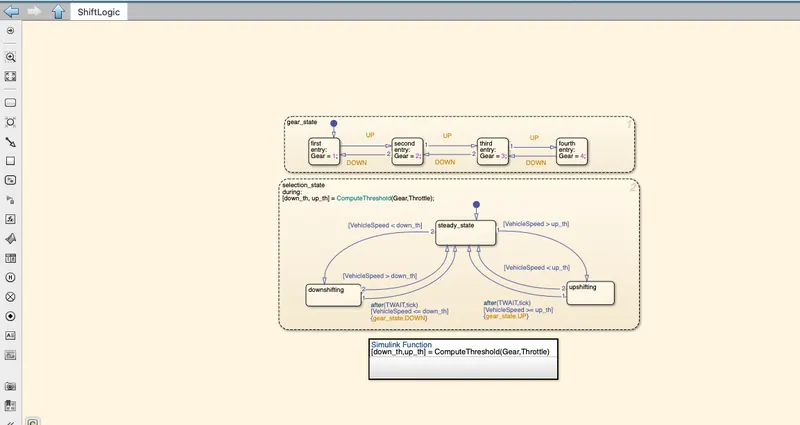
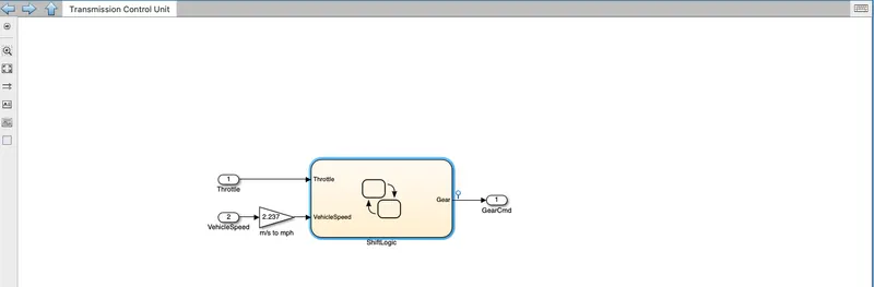
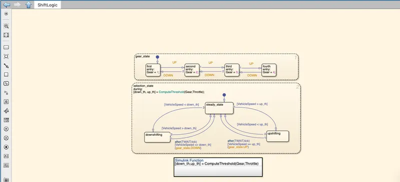
The transimision bloc is used to convert torque or speed.
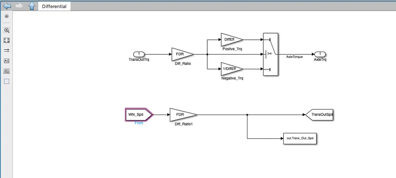
differential is usedTo help the engine power at the wheels. Transmit the power to the wheels as they rotate at a different speed. Act as final gear reduction in the vehicle by slowing the rotational speed of the transmission on final time before moving to the
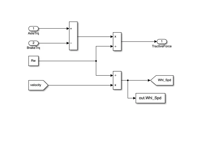
The automobile wheels support the total weight, resist the strains created during turning and transmit the driving torque for propelling and breaking torque for retarding. The wheels must have well balanced construction particularly for running at high speeds.
Considering the amount of complexity involved, it is the study of vehicle dynamics which plays a vital role in finding out the right balance between driver feel, comfort and safety of passengers and the fun and the wow factor which we all experience during driving
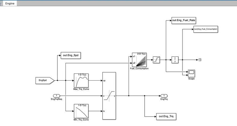
- The 2D lookup table is used to calculate the fuel flow rate based on engine speed and engine torque. The fuel flow rate is then integrated to find the fuel consumption
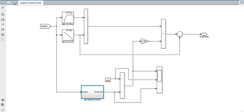
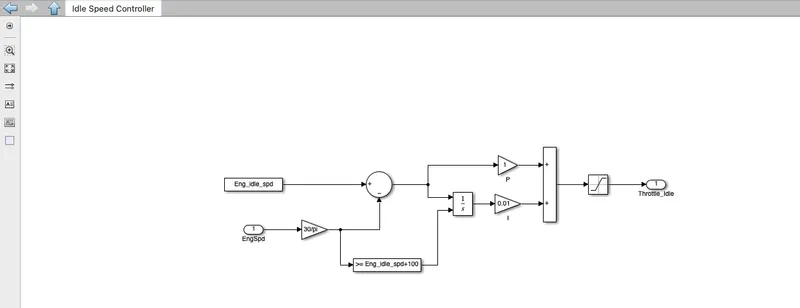
- Based on the Engine speed The required torque from the controller is saturated between Max torque curve and min torque curve and passes the Engine torque to the Transmission block
- Estimated fuel flow rate, fuel consumption, engine torque and engine speed are passed to the MATLAB workspace using the to-workspace block.
- Engine fuel flow rate and Fuel consumption are scoped.
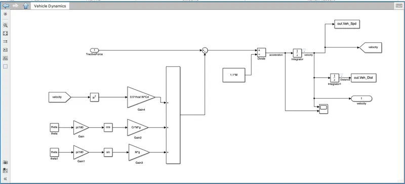
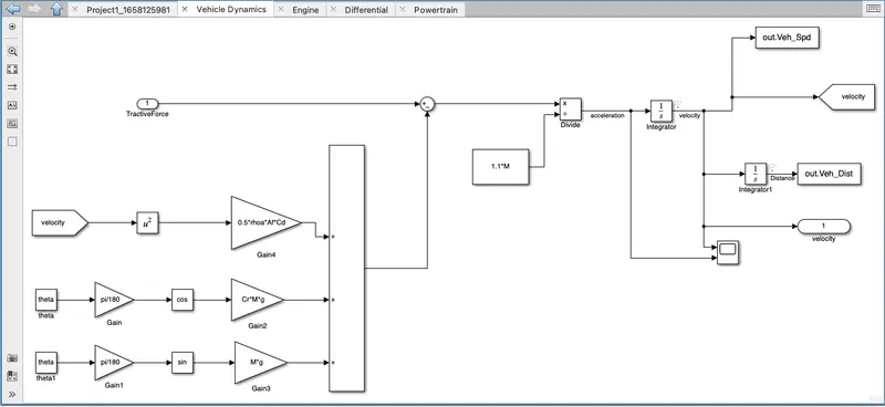
 The longitudinal dynamics of the vehicle along with the road load is represented in the Vehicle Dynamics’ block.
- Tractive Force and Road loads are used to calculate the vehicle velocity,
Where,
ρ a - Air Density
A f - Frontal Ares
C d - Drag Coefficient
C r - Rolling Coefficient
M - Mass of Vehicle
g - Acceleration due to gravity
θ - Slope
- The variables are loaded on the workspace using MATLAB Script.
- The Acceleration, Velocity and Distance travelled are Calculated and stored in the workspace.
%%%%%%%%%%%%%%%%%%%%%%%%%%%%%%%%%%%%%%%%%%%%%%%%%%%%%%%%%%%%%%%%%%%%%
%% Skill-Lync -> Hybrid Drives Development
% Project 1 - Conventional Vehicle Model
% By - Ullekh Gambhira
% Description:
% The following file is to used with the Initialization file and Simulink
% results for post-processing of the data.
% The file is incomplete, has some examples of how the data is imported
% into a readable format, data analysis and plotting examples.
% Based on the project task, use commands in a similar format as given
% below, to analyse the data and generate required plots.
% You can change variable names if desired
%% Post-Processing File
% File for post-processing the Conventional vehicle simulation model data
%% Renaming variables
Time = out.tout;
Acc_Pdl = out.Acc_Pdl; % Accelerator pedal [%]
Brk_Pdl = out.Brk_Pdl; % Brake pedal [%]
Gear_Cmd = out.Gear_Cmd; % Transmission gear
Trans_In_Spd = out.Trans_In_Spd*30/pi; % Transmission input speed [rpm]
Trans_Out_Spd = out.Trans_Out_Spd*30/pi;% Transmission output speed [rpm]
Eng_Trq = out.Eng_Trq; % Engine brake torque [Nm]
Eng_fuel_Rate = out.Eng_Fuel_Rate;
Eng_Spd = out.Eng_Spd*30/pi; % Engine speed [rpm]
Eng_Fuel_Consump = out.Eng_Fuel_Consumption; % Engine fuel consumption [g]
Veh_Dist = out.Veh_Dist/1000; % Distance traveled by vehicle [km]
Veh_Spd = out.Veh_Spd*18/5; % Vehicle speed [kmph]
%% Data Analysis
Eng_Pwr = Eng_Spd.*pi/30.*Eng_Trq/1000; % Engine brake power [kW]
rho_petrol = 0.7197; % Density of petrol [kg/L]
kmpl = Veh_Dist(end)./(Eng_Fuel_Consump(end)/1000/rho_petrol); % Fuel economy [kmpl]
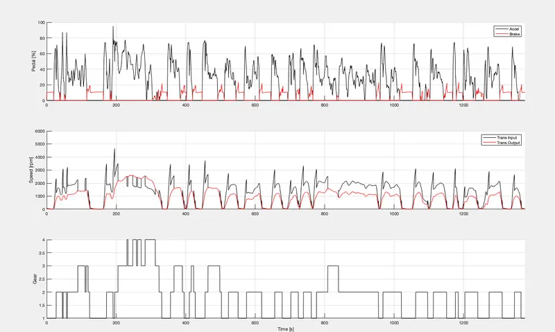
%% Plotting vehicle characteristics time trace
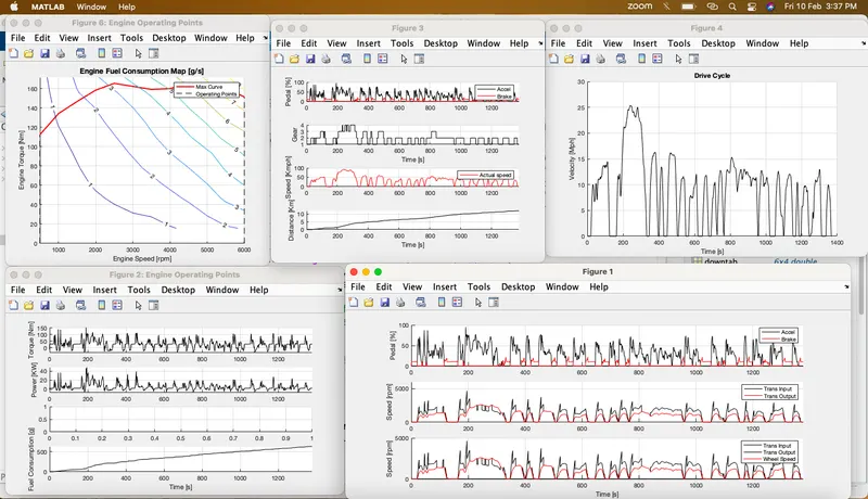
figure()
subplot(3,1,1)
hold on
grid on
plot(Time, Acc_Pdl, 'linewidth', 1, 'Color', 'black');
plot(Time, Brk_Pdl, 'linewidth', 1, 'Color', 'red');
ylabel('Pedal [%]')
xlim([0, Time(end)]);
legend('Accel','Brake');
subplot(3,1,2)
hold on
grid on
plot(Time, Trans_In_Spd, 'linewidth', 1, 'Color', 'black');
plot(Time, Trans_Out_Spd, 'linewidth', 1, 'Color', 'red');
ylabel('Speed [rpm]')
xlim([0, Time(end)]);
ylim([0, 6000]);
legend('Trans Input','Trans Output');
subplot(3,1,3)
hold on
grid on
plot(Time, Gear_Cmd, 'linewidth', 1, 'Color', 'black');
xlim([0, Time(end)]);
xlabel('Time [s]');
ylabel('Gear');
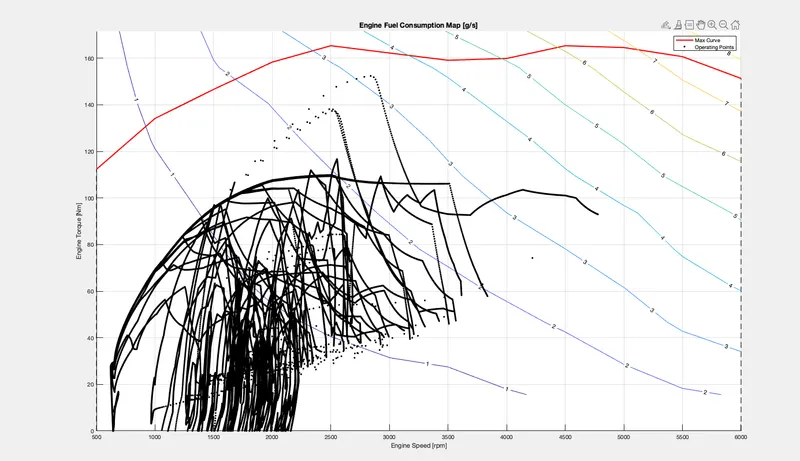
%% Plotting engine operating points on engine fuel map
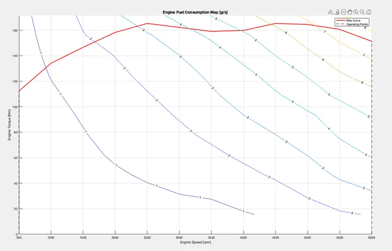
figure('Name','Engine Operating Points');
hold on
grid on
title('Engine Operating Points','fontsize',12);
p1=plot(Eng_map_spd*30/pi,Eng_max_trq,'linewidth',2,'color','r');
p2=line([Eng_map_spd(end)*30/pi Eng_map_spd(end)*30/pi],[0 Eng_max_trq(end)]);
set(p2,'linewidth',1,'linestyle','--','color','k');
p3=line([Eng_map_spd(1)*30/pi Eng_map_spd(1)*30/pi],[0 Eng_max_trq(1)]);
set(p3,'linewidth',1,'linestyle','--','color','k');
[c,h] = contour(Eng_map_spd'*30/pi,Eng_map_trq,Eng_fuel_map');
clabel(c,h);
xlabel('Engine Speed [rpm]');
ylabel('Engine Torque [Nm]');
title('Engine Fuel Consumption Map [g/s]');
p4 = plot(Eng_Spd,Eng_Trq,'.','color','k');
legend([p1 p4],{'Max Curve','Operating Points'});
axis([Eng_map_spd(1)*30/pi Eng_map_spd(end)*30/pi 0 Eng_map_trq(end)]);
%
%
%
%% Plotting vehicle characteristics time trace
% Plotting transmission input, transmission output and wheel speed
figure(1)
hold on
grid on
plot(Time, Trans_In_Spd, 'linewidth', 1, 'Color', 'black');
plot(Time, Trans_Out_Spd, 'linewidth', 1, 'Color', 'red');
xlabel('Time [s]')
ylabel('Speed [rpm]')
xlim([0, Time(end)]);
legend('Trans Input','Trans Output','Wheel Speed');
% Plotting engine torque, engine power, fuel rate and fuel consumption
figure(2)
subplot(4,1,1)
hold on
grid on
plot(Time, Eng_Trq, 'linewidth', 1, 'Color', 'black');
ylabel('Torque [Nm]')
xlim([0, Time(end)]);
subplot(4,1,2)
hold on
grid on
plot(Time, Eng_Pwr, 'linewidth', 1, 'Color', 'black');
ylabel('Power [KW]')
xlim([0, Time(end)]);
subplot(4,1,3)
hold on
grid on
subplot(4,1,4)
hold on
grid on
plot(Time, Eng_Fuel_Consump, 'linewidth', 1, 'Color', 'black');
xlim([0, Time(end)]);
xlabel('Time [s]');
ylabel('Fuel Consumption [g]');
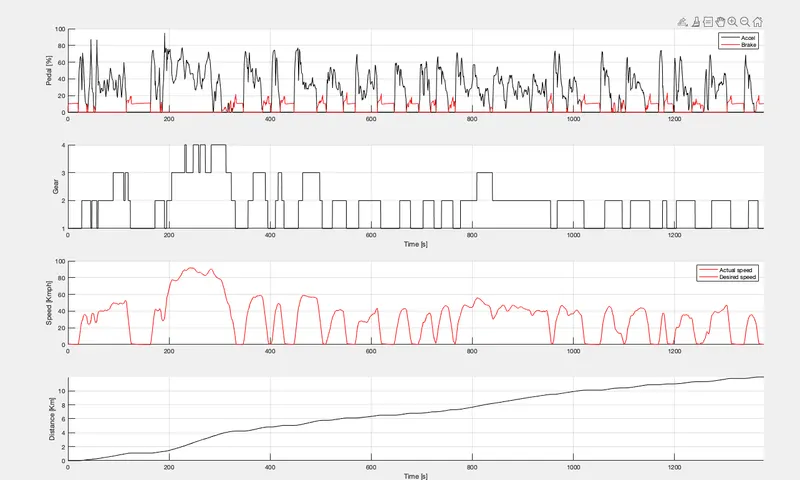
%Plotting accelerator and brake pedal gear command, vehicle desired and actual speed, vehicle distance
figure(3)
subplot(4,1,1)
hold on
grid on
plot(Time, Acc_Pdl, 'linewidth', 1, 'Color', 'black');
plot(Time, Brk_Pdl, 'linewidth', 1, 'Color', 'red');
ylabel('Pedal [%]')
xlim([0, Time(end)]);
legend('Accel','Brake');
subplot(4,1,2)
hold on
grid on
plot(Time, Gear_Cmd, 'linewidth', 1, 'Color', 'black');
xlim([0, Time(end)]);
xlabel('Time [s]');
ylabel('Gear');
subplot(4,1,3)
hold on
grid on
plot(Time, Veh_Spd, 'linewidth', 1, 'Color', 'red');
ylabel('Speed [Kmph]')
xlim([0, Time(end)]);
legend('Actual speed','Desired speed');
subplot(4,1,4)
hold on
grid on
plot(Time, Veh_Dist, 'linewidth', 1, 'Color', 'black');
xlim([0, Time(end)]);
xlabel('Time [s]');
ylabel('Distance [Km]');
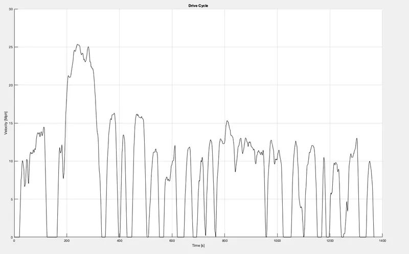
%% Plotting Drive Cycle
figure(4)
hold on
grid on
plot(cyc_time, cyc_vel, 'linewidth', 1, 'Color', 'black');
xlabel('Time [s]')
ylabel('Velocity [Mph]')
title('Drive Cycle')
% Test Results
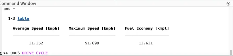
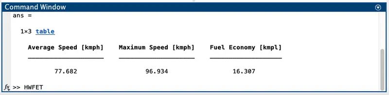
Avg_speed = sum(Veh_Spd)/length(Veh_Spd);
Max_Speed = maxk(Veh_Spd,1);
table(Avg_speed,Max_Speed,kmpl,'VariableNames',{'Average Speed [kmph]','Maximum Speed [kmph]','Fuel Economy [kmpl]'})
%% Plotting engine operating points on engine fuel map
figure('Name','Engine Operating Points');
hold on
grid on
title('Engine Operating Points','fontsize',12);
p1=plot(Eng_map_spd*30/pi,Eng_max_trq,'linewidth',2,'color','r');
p2=line([Eng_map_spd(end)*30/pi Eng_map_spd(end)*30/pi],[0 Eng_max_trq(end)]);
set(p2,'linewidth',1,'linestyle','--','color','k');
p3=line([Eng_map_spd(1)*30/pi Eng_map_spd(1)*30/pi],[0 Eng_max_trq(1)]);
set(p3,'linewidth',1,'linestyle','--','color','k');
[c,h] = contour(Eng_map_spd'*30/pi,Eng_map_trq,Eng_fuel_map');
clabel(c,h);
xlabel('Engine Speed [rpm]');
ylabel('Engine Torque [Nm]');
title('Engine Fuel Consumption Map [g/s]');
legend([p1 p3],{'Max Curve','Operating Points'});
axis([Eng_map_spd(1)*30/pi Eng_map_spd(end)*30/pi 0 Eng_map_trq(end)]);
%Tabulate the fuel economy numbers (kmpl) for UDDS and HWFET cycle. This
%forms the baseline numbers for comparing with the future hybrid version.