Project 1

%% Skill-Lync -> Hybrid Drives Development

% Project 1 - Conventional Vehicle Model

% By - Anku Vishwakarma

% Description:

%% Initialization File

% Initialization file for loading the variables for the Conventional vehicle simulation model

%% Vehicle Parameters

M = 1500; % Vehicle weight [kg]

Cr = 0.015; % Rolling resistance coefficient

Rw = 0.35; % Rolling radius [m]

Cd = 0.33; % Drag coefficient

Af = 2; % Frontal area [m2]

rhoa = 1.225; % Air density [kg/m3]

Vwind = 0; % Wind velocity [kmph]

g = 9.81; % Gravitational acceleration [m/s2]

theta = 0; % Slope [deg]

myu_road_tire = 1; % Coefficient of friction between tire - road interface

%% Powertrain Parameters

FDR = 3.73; % Final Drive Ratio / Diff Ratio

DiffEff = 0.99; % Differential efficiency (assumed independent of operating conditions)

NumGear = 4; % Number of gears in transmission

TransGear = 1:NumGear; % Transmission Gears

TransRatio = [3.06, 1.62, 1, 0.7]; % Corresponding Transmission ratios

TransEff = 0.90; % Transmission efficiency (assumed independent of operating conditions)

TC_SR = [0, .5, .6, .7, .8, .87, .92, .94, .96, .97, 1]; % Torque Converter Speed Ratio (Matlab default) -> TurbSpd/PumpSpd

TC_TR = [2.232, 1.5462, 1.4058, 1.2746, 1.1528, 1.0732, 1.0192, 1, 1, 1, 1]; % Torque Converter Torque Ratio (Matlab default) -> TurbTrq/PumpTrq

TC_Cf = 1e-4 * [.72558, .66322, .63463, .59042, .51331, .4144, .29287, .22444, .12186, .04386, 0]; % Torque Converter Capacity Factor (Matlab default) -> PumpTrq/PumpSpd^2 [Nm/rpm^2]

load Vehicle_Data/Engine_data_1_9L_Saturn_95kW

load Vehicle_Data/Trans_Shift_map

%% Driver Parameters

Kp = 10; % P gain for driver PI model

Ki = 1; % I gain for driver PI model

Drive_Cycle_Select = 1; % Drive cycle selection

% Drive cycle values in m/s

if Drive_Cycle_Select == 1

load DriveCycles/UDDS;

elseif Drive_Cycle_Select == 2

load DriveCycles/HWFET;

elseif Drive_Cycle_Select == 3

load DriveCycles/FTP;

elseif Drive_Cycle_Select == 4

load DriveCycles/US06;

elseif Drive_Cycle_Select == 5

load DriveCycles/NEDC;

elseif Drive_Cycle_Select == 6

load DriveCycles/WLTP;

end

time_end = cyc_time(end);

vel_end = cyc_vel(end);

Simulink blocks:-

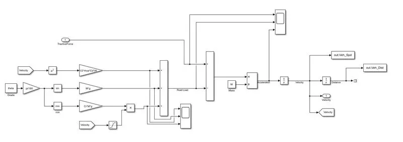
Simulink blocks of the engine and vehicle dynamics for the Simulink model

“Project1_VehicleModel.slx”

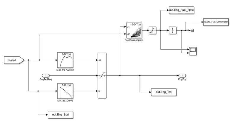
In the engine block, the input is the engine torque required and the output it gives is engine torque. The engine speed from the block is used whose signal is connected to two 1D lookup tables which have engine max torque and engine min torque as their table data. A saturation dynamic block is connected to both the signals of the lookup table and as an output, it gives engine torque.

Engine speed and engine torque are passed through a 2D lookup table and connected to a saturation block which then gives the engine fuel rate and after the signal passes through an integration block it gives engine fuel consumption.

Result -

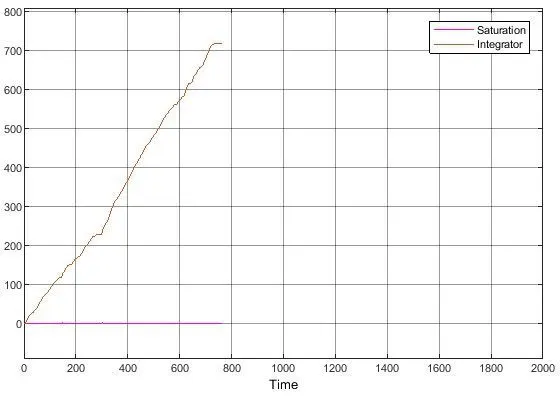
In the engine block scope result, it can be seen that as the vehicle moves forward the fuel rate remain constant but the fuel consumption gradually increases.

Result

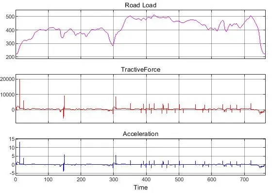
Below is the scope result for the vehicle dynamics block. Tractive force and acceleration have the same movement and the road load increases and decrease with the increase and decrease of the movement of tractive force and acceleration.

Project1_ProcessingFile.m

“Project1_ProcessingFile.m” is the Matlab script used to analyze this data and generate plots. This script needs to be executed after the Simulink model data has been loaded into the workspace. Here we rename the variables loaded from the model (if desired), do some basic post-process calculations, and generate results and plots.

The code has been modified as per the requirement. Plots for the engine outputs and vehicle dynamics have been added to the code using a Matlab code subplot.

Fuel economy (kmpl) for both UDDS and HWFET cycle is been calculated through the above code,

Drive Cycle UDDS

The EPA Urban Dynamometer Driving Schedule (UDDS) is commonly called the "LA4" or "the city test" and represents city driving conditions. It is used for light-duty vehicle testing. The UN/ECE Regulation 53 refers to the EPA UDDS as the "Test Equivalent to the Type 1 Test (verifying emissions after a cold start)."

Fuel economy is 14.2044 [kmpl]

Drive Cycle HWFET

The Highway Fuel Economy Driving Schedule (HWFET) represents highway driving conditions under 60 mph.

Fuel economy is 16.5010 [kmpl]

As per the fuel economy value for both cycles, the HWFET drive cycle has a higher economy than the UDDS drive cycle.

Plots:-

Drive Cycle UDDS

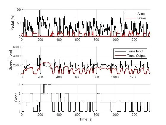
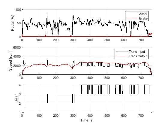
In the below plot, it can be seen that with an increase in gear, the accelerator pedal increases and there is no movement with the brake pedal. The speed increases with the moment of transmission input and output. Speed seems to be zero when there is movement in the brake pedal.

The vehicle reaches max gear only once in this cycle. The maximum time it is in 1st or 2nd gear.

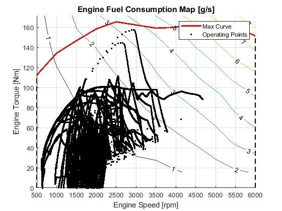
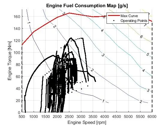
Operating points seem to be close to the max curve. Has less torque and speed compared to the UDDS drive cycle.

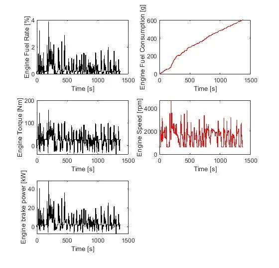
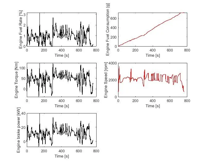
In this plot with an increase in torque, power increases, and when the decrease in torque, power also decreases. Both have a negative value as well. Engine fuel rate and speed plot have almost the same movement as the other plots. Engine fuel consumption gradually increases.

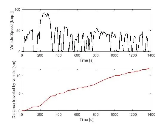
Lots of Up and down movement can be seen in the vehicle's speed, it reaches the maximum at one point and comes to zero at the next. This is how vehicle speed fluctuates in the UDDS drive cycle. Distance traveled by the vehicle plot is also not straight as compared to the HWFET drive cycle, it has some disturbance or some movement.

Drive Cycle HWFET

The brake pedal seems to be steady in the overall ride. Mostly the vehicle is at maximum gear and there is less movement in the accelerator pedal, only when there is a slight movement in the brake pedal. Less fluctuation is seen in the speed part for this drive cycle.

There is more torque generated with more engine speed. Operating points are away from the mas curve.

More power is generated in this drive cycle with more torque. A drastic change in the movement of the torque can be seen. There is less fluctuation in engine speed. Engine fuel consumption increases with time.

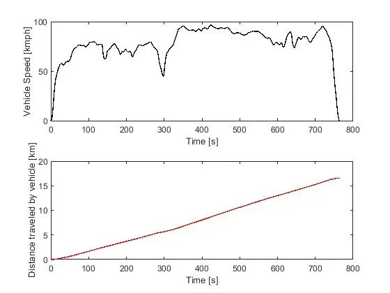
In the HWFET drive cycle, the distance traveled by the vehicle plot shows a straight line with no disturbance compared to the UDDS drive cycle. Vehicle speed increases from zero at the start of the vehicle and comes to the minimum when the vehicle stops. Very less movement can be seen throughout the ride.