Problem Set-1 c Week 11Challenge : Transient Handling
AIM :-
Using the given data calculate the following parameters,
- Undamped natural frequency.
- Damping ratio.
- Damped frequency.
- Rise time.
To plot the unit step response of the system for lateral speed, lateral acceleration and yaw rate.
To plot the sine response for lateral speed, lateral acceleration and yaw rate.
To plot the yaw gain in the frequency domain.
To show the correlation for the following,
- Steady state yaw gain between the sine response and frequency response plot.
- Yaw gain at 7 Hz between the sine response and frequency response plot.
- Response time between the step response plot and analytical calculations.
GIVEN DATA :-
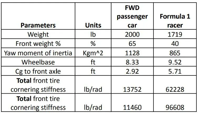
NUMERICAL SOLUTION :-
1. Calculate the Undamped Natural Frequency, Damping Ratio, Damped Frequency and Rise Time.
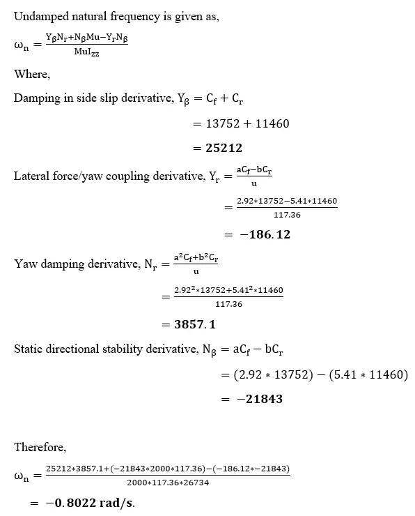
a) Undamped natural frequency.
The undamped frequency of the road car is,
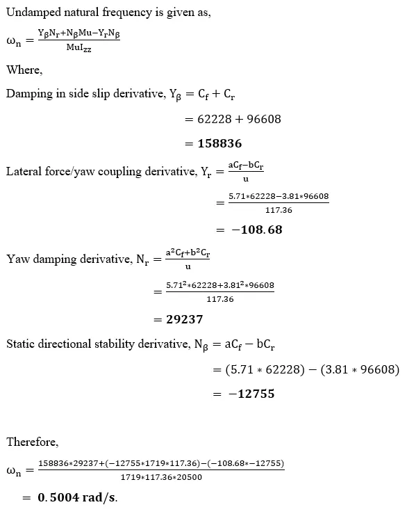
The undamped natural frequency of an F1 car is,
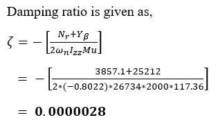
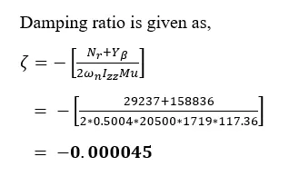
b) Damping ratio.
The damping ratio for a road car is,
The damping ratio for an F1 car is,
c) Dampend frequency.
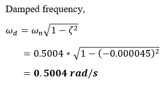
The damped frequency of a road car is,
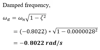
The damped frequency of an F1 car is,
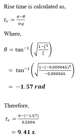
d) Rise time.
The rise time for a road car is,
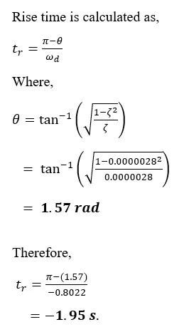
The rise time for an F1 car is,
MATLAB SCRIPT :-
In order to plot the graphs, MATLAB programs are written and the plots are obtained using state space representation.
The MATLAB script for the transient handling of a road car is given below.
% Transient handling of a passenger car.
clear all
close all
clc

% Inputs
M = 2000; % Weight of the car in lb.
Mf = 65*M/100; % Front weight distribution in lb.
Mr = M-Mf; % Rear weight distribution in lb.
Izz = 1128*23.7; % Yaw moment of inertia in lb-ft^2.
l = 8.33; % Wheelbase in ft.
a = 2.92; % Distance between CG and front axle in ft.
b = l-a; % Distance between CG and rear axle in ft.
Cf = 13752; % Front cornering stiffness in lb/rad.
Cr = 11460; % Rear cornering stiffness in lb/rad.
u = 80*1.467; % Vehicle speed in ft/s^2.

% Derivatives.
Yb = Cf+Cr; % Damping in side slip derivative.
Nr = ((a^2*Cf)+(b^2*Cr))/u; % Yaw damping derivative.
Nb = (a*Cf)-(b*Cr); % Static directional stability derivative.
Yr = ((a*Cf)-(b*Cr))/u; % Lateral force/yaw coupling derivative.

% Numerical calculations.
Wn = ((Yb*Nr)+(Nb*M*u)-(Yr*Nb))/(M*u*Izz); % Undamped natural frequency.
Zeta = -((Nr+Yb)/(2*Wn*(Izz*M*u))); % Damping ratio.
Wd = Wn*sqrt(1-Zeta^2); % Damped frequency.
theta = atan(sqrt(1-Zeta^2)/Zeta); % Angle for rise time.
Tr = (pi-theta)/Wd; % Rise time in seconds.

% State space matrix.
A = [-(Cf+Cr)/(M*u) , ((b*Cr-a*Cf)/(M*u))-u ;
     (b*Cr-a*Cf)/(Izz*u) , -(a^2*Cf+b^2*Cr)/(Izz*u)];

B = [Cf/M ; (a*Cf)/Izz];

C_lat = [1 , 0]; D_lat = 0; % Lateral speed.
C_yaw = [ 0 , 1]; D_yaw = 0; % Yaw rate.
C_acc = A(1,:); D_acc = B(1); % Lateral acceleration.

C = [C_lat ; C_yaw ; C_acc];
D = [D_lat ; D_yaw ; D_acc];

% Defining the time step.
t = 0:0.01:6;

U = (5*pi/180)*sin(7*2*pi*t); % 5 degrees of steering input at 7 Hz.

sys = ss(A,B,C,D); % State space representation.
Y = lsim(sys,U,t); % Sinusoidal input.

sys.inputname = {'Steering'};
sys.outputname = {'lat' ; 'yaw' ; 'acc'};

% Plotting the graphs

figure(1) % Frequency response
[mag,w] = bodemag(sys({'yaw'},'Steering'));
loglog(w/6.28,[mag],'linewidth',3);
grid on;
title('Yaw rate/steer angle frequency response');
xlabel('Frequency (Hz)');
ylabel('Yaw rate (deg/s)');

figure(2) % Step response.
step(sys);
grid on;

figure(3) % Sine response.
subplot(2,2,1);
grid on;
plot(t,Y(:,1),'linewidth',3);
title('Lateral speed');
xlabel('Time (s)');
ylabel('Lateral speed (m/s)');

subplot(2,2,2);
grid on;
plot(t,Y(:,2)*180/pi,'linewidth',3);
title('Yaw rate');
xlabel('Time (s)');
ylabel('Yaw rate (deg/s)');

subplot(2,2,3);
grid on;
plot(t,Y(:,3),'linewidth',3);
title('Lateral acceleration');
xlabel('Time (s)');
ylabel('Lateral acceleration (m/s^2)');

subplot(2,2,4);
grid on;
plot(t,U*180/pi,'linewidth',3);
title('Steering angle');
xlabel('Time');
ylabel('Steering angle (deg)');
The MATLAB script for the transient handling of an F1 car is given below,
% Transient handling of an F1 car.
clear all
close all
clc

% Inputs
M = 1719; % Weight of the car in lb.
Mf = 40*M/100; % Front weight distribution in lb.
Mr = M-Mf; % Rear weight distribution in lb.
Izz = 865*23.7; % Yaw moment of inertia in lb-ft^2.
l = 9.52; % Wheelbase in ft.
a = 5.71; % Distance between CG and front axle in ft.
b = l-a; % Distance between CG and rear axle in ft.
Cf = 62228; % Front cornering stiffness in lb/rad.
Cr = 96608; % Rear cornering stiffness in lb/rad.
u = 80*1.467; % Vehicle speed in ft/s^2.

% Derivatives.
Yb = Cf+Cr; % Damping in side slip derivative.
Nr = ((a^2*Cf)+(b^2*Cr))/u; % Yaw damping derivative.
Nb = (a*Cf)-(b*Cr); % Static directional stability derivative.
Yr = ((a*Cf)-(b*Cr))/u; % Lateral force/yaw coupling derivative.

% Numerical calculations.
Wn = ((Yb*Nr)+(Nb*M*u)-(Yr*Nb))/(M*u*Izz); % Undamped natural frequency.
Zeta = -((Nr+Yb)/(2*Wn*(Izz*M*u))); % Damping ratio.
Wd = Wn*sqrt(1-(Zeta^2)); % Damped frequency.
theta = atan(sqrt(1-Zeta^2)/Zeta); % Angle for rise time.
Tr = (pi-theta)/Wd; % Rise time in seconds.

% State space matrix.
A = [-(Cf+Cr)/(M*u) , ((b*Cr-a*Cf)/(M*u))-u ;
     (b*Cr-a*Cf)/(Izz*u) , -(a^2*Cf+b^2*Cr)/(Izz*u)];

B = [Cf/M ; (a*Cf)/Izz];

C_lat = [1 , 0]; D_lat = 0; % Lateral speed.
C_yaw = [ 0 , 1]; D_yaw = 0; % Yaw rate.
C_acc = A(1,:); D_acc = B(1); % Lateral acceleration.

C = [C_lat ; C_yaw ; C_acc];
D = [D_lat ; D_yaw ; D_acc];

% Defining the time step.
t = 0:0.01:6;

U = (5*pi/180)*sin(7*2*pi*t); % 5 degrees of steering input at 7 Hz.

sys = ss(A,B,C,D); % State space representation.
Y = lsim(sys,U,t); % Sinusoidal input.

sys.inputname = {'Steering'};
sys.outputname = {'lat' ; 'yaw' ; 'acc'};

% Plotting the graphs

figure(1) % Frequency response
[mag,w] = bodemag(sys({'yaw'},'Steering'));
loglog(w/6.28,[mag],'linewidth',3);
grid on;
title('Yaw rate/steer angle frequency response');
xlabel('Frequency (Hz)');
ylabel('Yaw rate (deg/s)');

figure(2) % Step response.
step(sys);
grid on;

figure(3) % Sine response.
subplot(2,2,1);
grid on;
plot(t,Y(:,1),'linewidth',3);
title('Lateral speed');
xlabel('Time (s)');
ylabel('Lateral speed (m/s)');

subplot(2,2,2);
grid on;
plot(t,Y(:,2)*180/pi,'linewidth',3);
title('Yaw rate');
xlabel('Time (s)');
ylabel('Yaw rate (deg/s)');

subplot(2,2,3);
grid on;
plot(t,Y(:,3),'linewidth',3);
title('Lateral acceleration');
xlabel('Time (s)');
ylabel('Lateral acceleration (m/s^2)');

subplot(2,2,4);
grid on;
plot(t,U*180/pi,'linewidth',3);
title('Steering angle');
xlabel('Time');
ylabel('Steering angle (deg)');
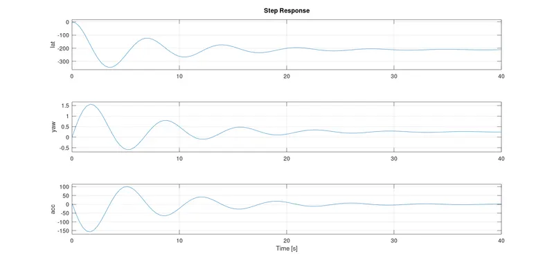
2. Plot the Unit Step Response of the System for Lateral Speed, Yaw Rate and Lateral Acceleration.
The step response of a road car is given below.
The step response of an F1 car is given below.
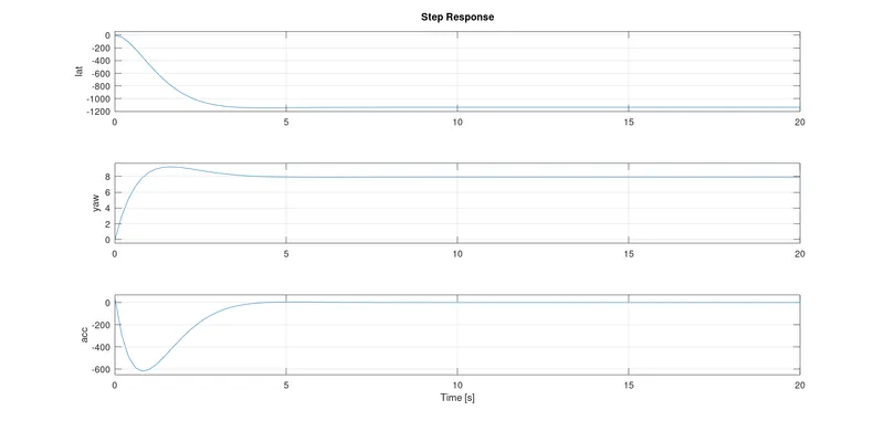
From the plots of the road car and the F1 car, the lateral acceleration is negative in both cases. The damping in an F1 car is much greater than a road car, where the oscillations are higher in car of the road car's step response plots.
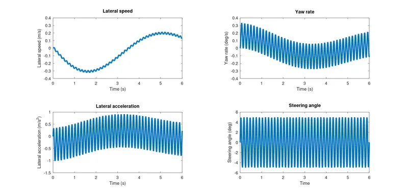
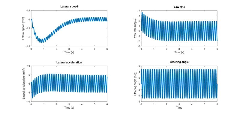
3. Plot the Sine Response for Lateral Speed, Yaw Rate and Lateral Acceleration for 5 degrees of Steering Input at 7 Hz.
The sine response for a road car is given below.
The sine response for an F1 car is given below.
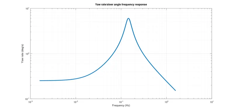
4. Plot the Yaw Gain in the Frequency Response.
The frequency response of a road car is given below.
The frequency response of an F1 car is given below.
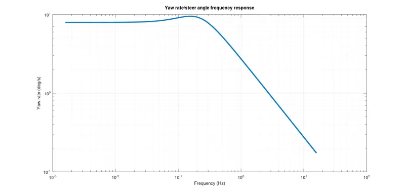
The plots of the frequency response indicate that the F1 car has a much sharper steering response for 5 degrees of steering input at 7 Hz.