PLOTTING AIR STANDARD OTTO CYCLE USING MATLAB
AIR STANDARD OTTO CYCLE
1. AIM:
To plot Pressure v/s volume graph of Air Standard Cycle (otto cycle) using MATLAB.
2. GOVERNING EQUATION:
The Otto cycle is an air-standard cycle which approximates the processes in petrol or diesel engines. It is based on constant volume heat addition (combustion) and heat rejection processes, and Isentropic compression and expansion.
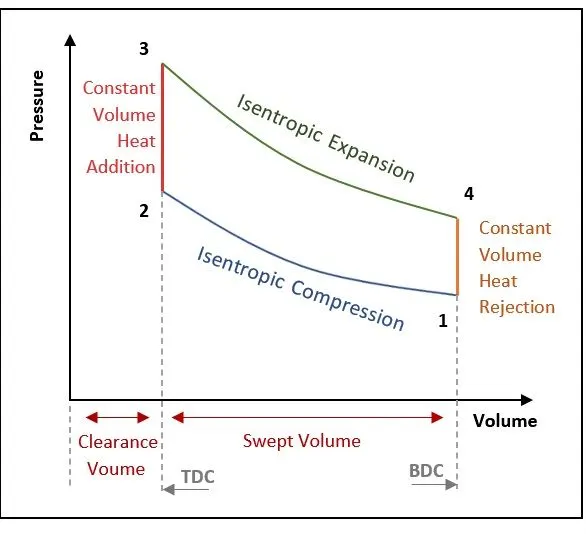
Figure.1 Otto cycle PV graph diagram
Processes:
1 - 2 Isentropic compression
2 - 3 Constant volume heat addition
3 - 4 Isentropic Expansion
4 - 1 Constant volume heat rejection
- For Isentropic process 1-2 and 3-4 ,
p1v1^γ = p2v2^γ and (p1v1)/t1 = (p2v2)/t2
where number indicate the process state
Same equation is used in the other process state also.
- Assumption: 1. Sq. heat ratio γ = 1.4
2. Temp. from compression t3 = 2500K
3. p1 = 101325 Pa
4. t1 = 600 K
- Geometric parameter: 1. Bore Diameter = 0.2
2. Stroke = 0.2
3. connecting rode length = 0.22
4. Compression ratio (cr) = 12
5. v/vc = 1+1/2(cr-1)[R+1-cosθ-(R^2 − sin^2θ )^1/2)]
where θ is crank angle
- thermal efficiency = 1-1/crγ-1
3. OBJECTIVES OF THE PROJECT:
- To plot Pressure v/s Volume graph of Air Standard Cycle (Otto Cycle) using MATLAB.
- To find the Thermal Efficiency of engine.
4. FLOW OF PROJECT:
- Assume intial values of Pressure and Temperature and engine geometric parameters
- Calculate the value of Pressure and Temperature of different state of the cycle ie, 1 to 4 using appropriate equations of different types pf process.
- Plot the graph mentioned in the objectives.
- Find the thermal efficiency
5. MATLAB CODE:
Program 1: Function code
%function code named 'ottocycle_function' have output is volume(v) and input parameters are bore length, stroke length, connecting rode length, compression ratio(cr),swept and clearance volume, starting and ending crank.
function [V] = ottocycle_function(bore,stroke,cond_rode,cr,start_crank,end_crank);

%geometric functions
a = stroke/2;
R = cond_rode/a;

%swept and clearance volume
v_swept = (pi/4)*bore^2*stroke;
v_clear = v_swept/(cr-1);

%angle
theta = linspace(start_crank,end_crank,100);

%volume trace equation
term1 = 0.5*(cr-1);
term2 = R+1-cosd(theta);
term3 = (R^2-sind(theta).^2).^0.5;

 V = (1+term1*(term2-term3)).*v_clear;

end
Program 2: Main code by using function
%program for the Air standard cycle

clear all
close all
clc

%inputs
gamma = 1.4;
t3 = 2500;

%state variable at 1
p1 = 101325;
t1 = 600;

%engine geometric parameter
bore = 0.2;
stroke = 0.2;
cond_rode = 0.22;
cr = 12;

%swept and clearance volume
v_swept = (pi/4)*bore^2*stroke;
v_clear = v_swept/(cr-1);

v1 = v_swept + v_clear;
v2 = v_clear;

%state variable at 2
%p1v1^gamma = p2v2^gamma
p2 = p1*cr^gamma;

%p1v1/t1 = p2v2/t2
t2 = p2*v2*t1/(p1*v1);
constant_c = p1*v1^gamma;
v_comp = ottocycle_function(bore,stroke,cond_rode,cr,180,0);
p_comp = constant_c./(v_comp.^gamma);

%state variable at 3
v3 = v2;

%p3v3/t3 = p2v2/t2 | p3 = p2v2t3/(t2v3)
p3 = p2*t3/t2;
constant_c = p3*v3^gamma;
v_exp = ottocycle_function(bore,stroke,cond_rode,cr,0,180);
p_exp = constant_c./(v_exp.^gamma);

%state variable at 4
v4 = v1;

%p3v3^gamma = p4v4^gamma | p4 = p3v3/v4^gamma
p4 = p3*(v3/v4)^gamma;

%thermal efficiency
thermal_eff = 1-(1/(cr^(gamma-1)));
final_eff = thermal_eff*100+"%"

%plotting
figure(1)
hold on;
grid on;
plot(v1,p1,'*','color','r');
plot(v_comp,p_comp);
plot(v2,p2,'*','color','r');
plot(v3,p3,'*','color','r');
plot(v_exp,p_exp);
plot(v4,p4,'*','color','r');
plot([v2,v3],[p2,p3],'color','b');
plot([v4,v1],[p4,p1],'color','b');

xlabel('Volume(v)');
ylabel('Pressure(p)');

%figure(2)
%plot([v1,v2,v3,v4],[p1,p2,p3,p4],'color','b');
6. OBSERVATION:
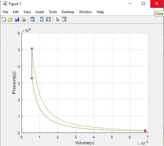
Figure.2 Output PV graph
7. ERROR FACED:
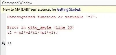
- While programming instead of intial value temperature at state 1 (t1) , mention value of temperature at state 2 (t2).
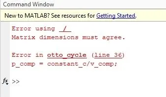
- Forget to give matrix dimension in equation 'p_com = constant_c/v_comp' because v_comp is in the array form.
8. CONCLUSION:
- Plotted PV graph of Otto cycle in MATLAB.
- Obtained thermal efficiency
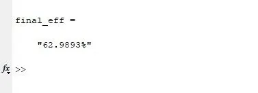
Figure.3 Thermal Efficiency