Otto cycle simulation

Aim: Write code for solving otto cycle and generate plots

Objective:

• To create Pressure-Volume Diagram of Otto cycle
• Calculate the Thermal efficiency of the engine

Problem Statement:

• Otto cycle is an ideal thermodynamics cycle; it tells how the heat engines work and how the gasoline is converted into energy and then into motion. The PV diagram of otto cycle shows how the changes in pressure and volume of the working fluid change due to the combustion of hydrocarbons which powers movements of piston, creating heat to provide motion for a vehicle.

Equation:

`V=(1+(1/2)(cr-1)[R+1 - cos⁡θ-( R^2- sin^2(theta ))^(1/2) ])*V_c`

where,

V = Volume, m^3

cr = Compression ratio

R = Ration of connecting rod length and crank pin radius

`theta` = Crank angle, degrees

V_c = Clearance volume, m^3

• Based on the concepts of Forward Kinematics, write a code to solve Otto cycle and find the Thermal efficiency.

Solution Procedure:

• Import ‘math’ and ‘matplotlib’ modules.
• Define function ‘engine_kinematics’ to calculate Compression and Expansion Volume.
• Calculate swept volume and clearance volume, from which volumes of state points 1 and 2 are obtained.
• Define Inputs such as gamma - specific heat ratio of gas, and some state variables such as t3 - temperature at state point 3, p1 and t1 – pressure and temperature at state point 1 respectively.
• Then the engine geometric parameters are defined such as bore diameter, stroke length, connecting rod length and compression ratio which is ratio of volumes of state point 1 and 2 or state point 4 and 3.
• Calculate the state point variables of 2,3 and 4 such as p2,t2,v3,p3,v4,p4 and t4.
• Call function ‘engine_kinematics’ to obtain compression and expansion volume.
• Where Compression and Expansion values of Pressure has been calculated using the ideal gas equation.
• Then the state points have been plotted using the values of volume and pressure of different state points
• The isentropic compression and expansion curves has been plotted using the values of compression and expansion of both volume and pressure
• Then the isochoric heat addition and rejection curves are plotted using the state points, here the curve is straight line
• Then the title and axis labels are given
• Lastly the Thermal efficiency is calculated, whose value depends on the compression ratio

Code:

# Program to plot PV diagram of otto cycle and calculate Thermal efficiency of otto cycle

import math
import matplotlib.pyplot as plt

# Function to calculate volume 
def engine_kinematics(bore,stroke,con_rod,cr,start_crank,end_crank):
	# Engine Kinematics
	# Geometric Parameters
	a = stroke/2 	# crank pin radius
	R = con_rod/a  	# ratio of 'connecting rod length' and 'crank pin radius'

	# Calculating the Swept volume(V_s) and the Clearance volume(V_c)
	V_s = math.pi*(1/4)*pow(bore,2)*stroke
	V_c = V_s/(cr-1)

	sc = math.radians(start_crank)
	ec = math.radians(end_crank)

	num_values = 50

	dtheta = (ec-sc)/(num_values-1)

	V = []

	for i in range (0,num_values):
		theta = sc + i*dtheta
		term1 = 0.5*(cr-1)
		term2 = R + 1 - math.cos(theta)
		term3 = pow(pow(R,2) - pow(math.sin(theta),2),0.5)
		V.append((1 + term1*(term2-term3))*V_c)
	return V

# inputs
p1 = 101325
t1 = 500
gamma = 1.4
t3 = 2300

# geometric parameters
bore = 0.1       # Bore diameter,m
stroke = 0.1     # Stroke length,m
con_rod = 0.15   # Connecting rod length,m
cr = 8           # Compression ratio

# Volume computation
v_s = (math.pi/4)*pow(bore,2)*stroke
v_c = v_s/(cr-1)
v1 = v_c + v_s

# state point 2
v2 = v_c

# p2v2^gamma = p1v1^gamma
p2 = p1*pow(v1,gamma)/pow(v2,gamma)

# p2v2/t2 = p1v1/t1 | rhs = p1v1/t1 | p2v2/t2 = rhs | t2 = p2*v2/rhs
rhs = p1*v1/t1
t2 = p2*v2/rhs
V_compression = engine_kinematics(bore,stroke,con_rod,cr,180,0)
constant = p1*pow(v1,gamma)
P_compression = []

for v in V_compression:
	P_compression.append(constant/pow(v,gamma))


# state point 3
v3= v2

# p3v3/t3 = p2v2/t2 | rhs = p2v2/t2 | p3 = rhs*t3/v3
rhs = p2*v2/t2
p3 = rhs*t3/v3

V_expansion = engine_kinematics(bore,stroke,con_rod,cr,0,180)
constant = p3*pow(v3,gamma)
P_expansion = []

for v in V_expansion:
	P_expansion.append(constant/pow(v,gamma))

# state point 4
v4 = v1

# p4v4^gamma = p3v3^gamma
p4 = p3*pow(v3,gamma)/pow(v4,gamma)

# p4v4/t4 = rhs
t4 = p4*v4/rhs

# Plotting PV diagram
plt.plot(v1,p1,'*')                   # State point 1
plt.plot(v2,p2,'*')                   # State point 2
plt.plot(v3,p3,'*')                   # State point 3
plt.plot(v4,p4,'*')                   # State point 4
plt.plot(V_compression,P_compression) # Isentropic compression curve
plt.plot(V_expansion,P_expansion)     # Isentropic expansion curve 
plt.plot([v2,v3],[p2,p3])             # Isochoric heat addition curve
plt.plot([v4,v1],[p4,p1])             # Isochoric heat rejection curve 
plt.title("PV diagram of Otto cycle")
plt.xlabel("Volume")
plt.ylabel("Pressure")
plt.show()

# Calculating Thermal efficiency of otto cycle
Thermal_efficiency = 1-1/(pow(cr,(gamma-1)))
print("Thermal efficiency = ",Thermal_efficiency)

Results:

1. PV diagram:-

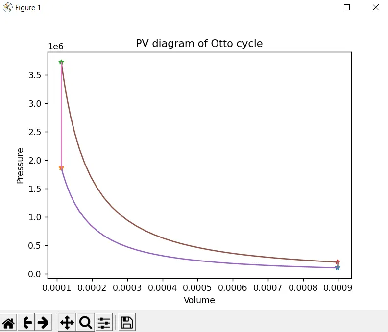
• Above figure is the graphical representation of the changes in pressure with respect to volume in a system
• The four points in the above figure represents four states of gas with values of volume and pressure
• The four states are,

(1). 1-2 Isentropic compression

(2). 2-3 Isochoric heat addition

(3). 3-4 Isentropic expansion

(4). 4-1 Isochoric heat rejection

2. Output of Thermal efficiency

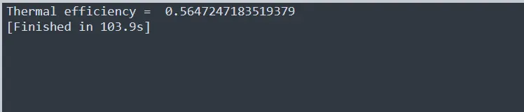
• Above figure shows the output of Thermal efficiency of the engine
• The thermal efficiency of the engine depends on the compression ratio of the engine

Discussion:

• The PV diagram has been plotted for the Otto cycle
• The Thermal efficiency of the engine has been generated