Week 4.1 - Optimizing Stalagmite Function using Genetic Algorithm in MATLAB
The stalagmite is a special type rock that usually formed inside the cave. The stalagmite normally rises from the floor. The rock formed because of the accumulation of the materials on the floor from the dripping of the ceilings.
The stalagmite function got name from this particular rock because of the similarity with the surface graph produced by this function. The stalagmite function has been represented by the following 3 dimensional equations,
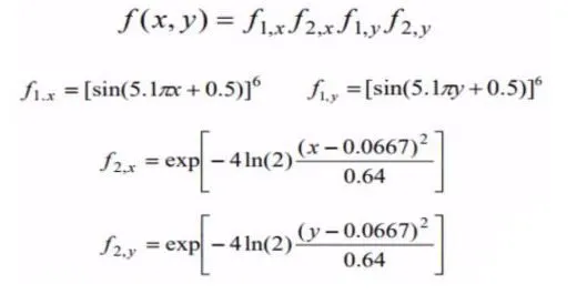
The objective of the current challenge is to optimize the above mentioned function by finding the global optima using the Genetic Algorithm using the MATLAB.
Main Code:
% Writing program for optimizing the stalagmite function using the Genetic
% Algorithm. The objective is to find the global optimum point of
% stalagmite function.

% The program will be coded for the unbounded search space, bounded search
% space & the third one by oincreasing the population size.
% The optimization time wil be measured for each study to compare with each
% other & to find the most efficienct way to use the GA to solve
% optimization problem.

% Solve = Genetic Algorithm (GA)


close all; clear all; clc;

% Inputs of the Problem
x = linspace(0,0.6,150);
y = linspace(0,0.6,150);
num_spaces = 50;

[xx, yy] = meshgrid(x,y); % Generating 2D Mesh
for i = 1:length(xx)
    for j = 1:length(yy)
        input_vector(1) = xx(i,j);
        input_vector(2) = yy(i,j);
        f(i,j) = stalagmite_function(input_vector);
    end
end

% (1) Program for Unbounded Space
tic % Starting stopwatch timer to measure optimization time
for i = 1:num_spaces
    % Calling stalagmite function using ga solver
    [results, fopt(i)] = ga(@stalagmite_function,2); % 2 = number of variables
    xopt(i) = results(1);
    yopt(i) = results(2);
end
program1 = toc % Reading elapsed time in stopwatch

% Plotting
figure(1)
subplot(2,1,1)
hold on
surfc(x,y,-f) % Plotting surface plot
shading interp % Setting shading color option as Interpolated
% Plotting 3d line plot
plot3(xopt, yopt, -fopt, 'marker', 'o')
subplot(2,1,2)
plot(-fopt)
xlabel('Iterations')
ylabel('Function Max')
title('Unbounded Space')

% (2) Program for Bounded Space
tic % Starting stopwatch timer to measure optimization time

lb = [0 0]; % Lower Bound
ub = [0.6 0.6]; % Upper Bound
for i = 1:num_spaces
    % Calling stalagmite function using ga solver
    [results, fopt(i)] = ga(@stalagmite_function,2,[],[],[],[],lb,ub); % 2 = number of variables
    xopt(i) = results(1);
    yopt(i) = results(2);
end
program2 = toc % Reading elapsed time in stopwatch

% Plotting
figure(2)
subplot(2,1,1)
hold on
surfc(x,y,-f) % Plotting surface plot
shading interp % Setting shading color option as Interpolated
% Plotting 3d line plot
plot3(xopt, yopt, -fopt, 'marker', 'o')
subplot(2,1,2)
plot(-fopt)
xlabel('Iterations')
ylabel('Function Max')
title('Bounded Space')

% (3) With High Number of Intial Population
lb = [0 0]; % Lower Bound
ub = [0.6 0.6]; % Upper Bound

% GA Options
options = optimoptions('ga', 'PopulationSize', 300);
tic % Starting stopwatch timer to measure optimization time
for i = 1:num_spaces
    % Calling stalagmite function using ga solver
    [results, fopt(i)] = ga(@stalagmite_function,2,[],[],[],[],lb,ub, ...
        [],[],options);
    xopt(i) = results(1);
    yopt(i) = results(2);
end
program3 = toc % Reading elapsed time in stopwatch

% Plotting
figure(3)
subplot(2,1,1)
hold on
surfc(x,y,-f) % Plotting surface plot
shading interp % Setting shading color option as Interpolated
% Plotting 3d line plot
plot3(xopt, yopt, -fopt, 'marker', 'o')
subplot(2,1,2)
plot(-fopt)
xlabel('Iterations')
ylabel('Function Max')
title('Bounded Inputs with High Initial Poplution Size')
Stalagmite Function:
function [s] = stalagmite_function(input_vector)

% The function is for the stalagmite optimization problem.
% The function will return the single value for both x & y.
x = input_vector(1);
y = input_vector(2);

% Equations
f1x = (sin(5.1*pi*x + 0.5)).^6;
f2x = exp(-4*log(2)*(((x - 0.0667).^2)/0.64));

f1y = sin(5.1*pi*y +0.5).^6;
f2y = exp(-4*log(2)*(((y - 0.0667).^2)/0.64));

% By default GA, search for the gloabal minima point. But the objective is
% to find the global maxima, thats why the function will be negative to
% indicate the solver to search the space opposite way.
[s] = -(f1x.*f1y.*f2x.*f2y);

end
Results:
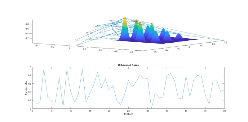
1) Unbounded Space
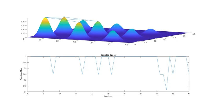
2) Bounded Space
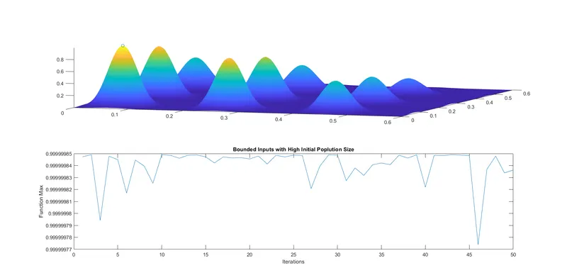
3. Bounded Space with Increased Population Size
4) Comparing Computation time taken by each method
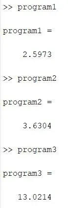
As we can see that the computation time taken by the bounded space with increased population size is very high compare to other two methods.