Mixing Tee in Ansys Fluent

Aim : To simulate the airflow through a mixing tee and observe the results in Ansys Fluent.

Objective : A Mixing Tee geometry is considered in this Project where I would simulate the airflow from 2 inlets and there is an outlet. There are multiple cases where the speed of airflow is changed or the size of pipe is altered to see the effect on the results.

Introduction : First the geometry is loaded in the Space claim and names are alloted to the 2 inlets, an outlet and walls. Initially we had a shell model so hide it in order to only focus on the wet volume. The physics for the shell (at the inlets and outlet) is supressed.

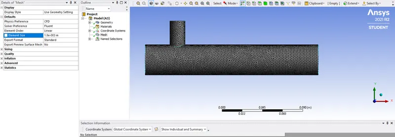
Then we load the geometry in the Mesh module where we provide an optimum mesh element size value so that we get a refined mesh. Here I took a Element size of `2e-3` = 0.002. Then we load the geometry in the setup module where we can check the mesh quality. Here we select the solver for the physics we are solving for this geometry. I have used Pressure based solver and performing steady state simulation. The model i am using to solve is realizable `K-epsilon` model with standard wall functions. The fluid is air. Then we define the boundary conditions with inlet and outlet air flow velocity and temperature and outlet pressure. The outlet pressure is set at gauze pressure as 0. The plots we want will also be added in tabs like residuals , area weighted average temperature , standard temperature deviation. And we will observe after how many iterations we get a converged result. Then we move on to next module where we do post processing and observe the result in a rainbow plane where we can see the results coloured format.

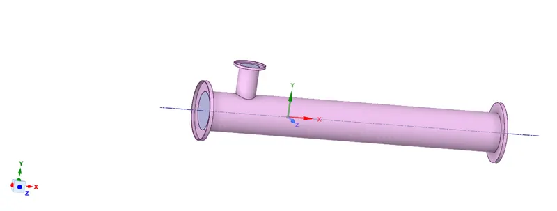
the geometry is given as follows :

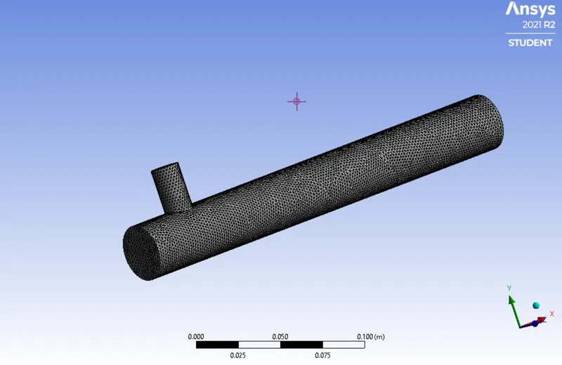
The meshed results as follows :

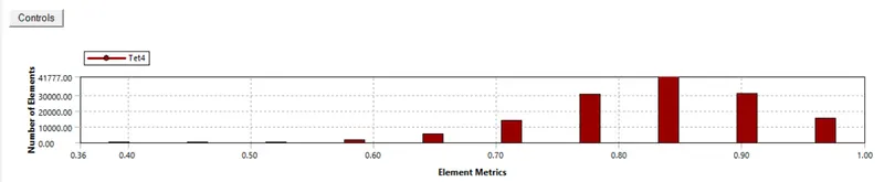
for mesh quality we can check in the mesh metrics parameter. the value should not fall below 40 percent.

Case 1 :
Here we consider the flow velocity from inlet along x axis as 3 m/s and along y-axis as 6. That is a momentum ratio of 2.

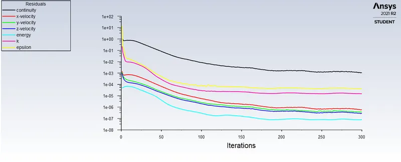
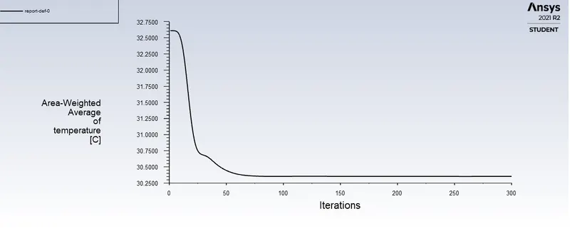
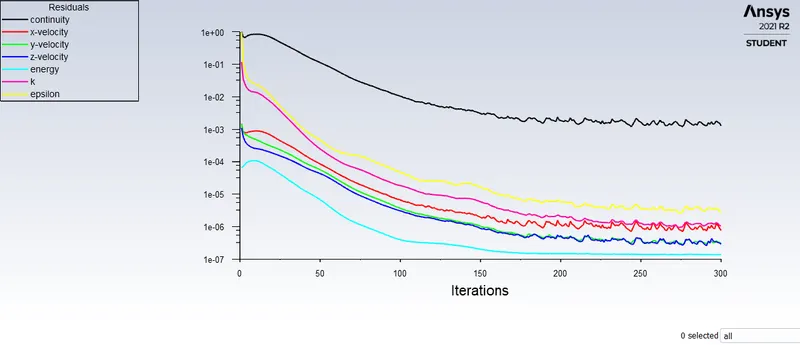
We solve the Navier Stokes equation for 300 iterations and see the results as follows :

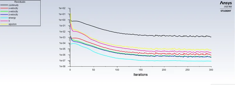
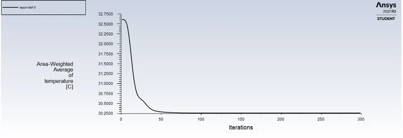
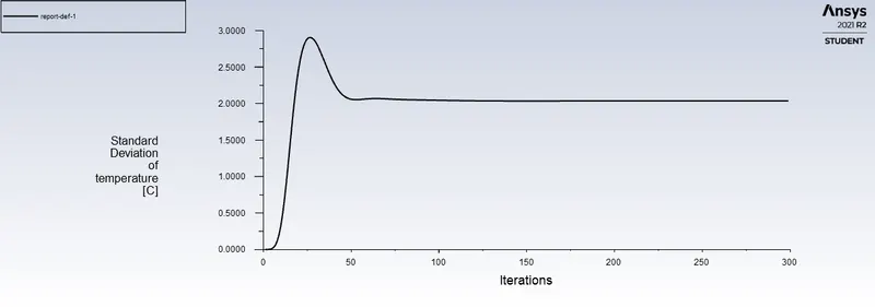
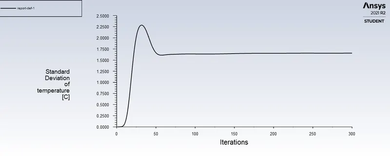
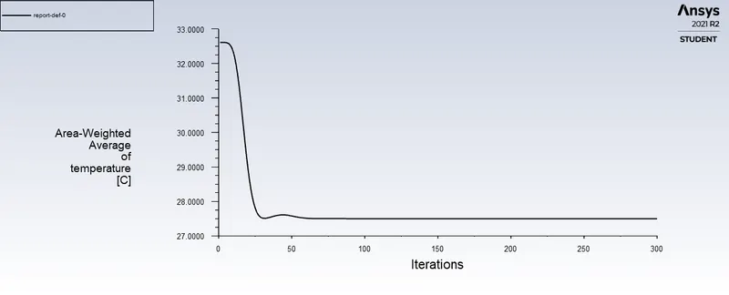
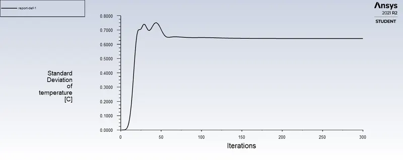
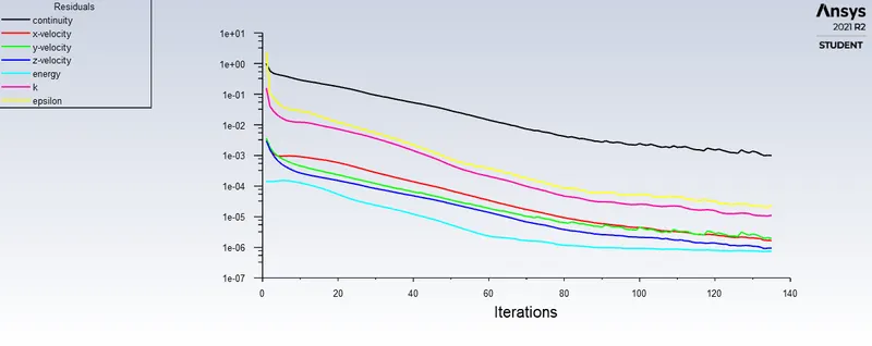
we observe from the above graphs how the results converged after 150 iterations. And the area weighted average and standard deviation for temperature also converged after 50 iterations.

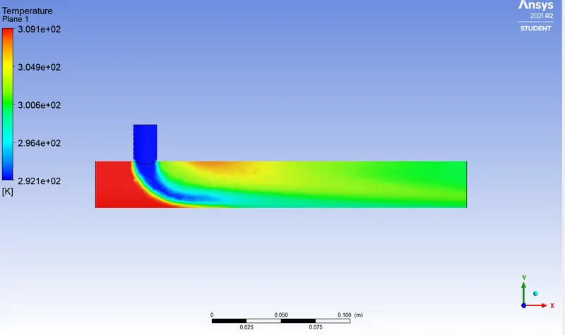
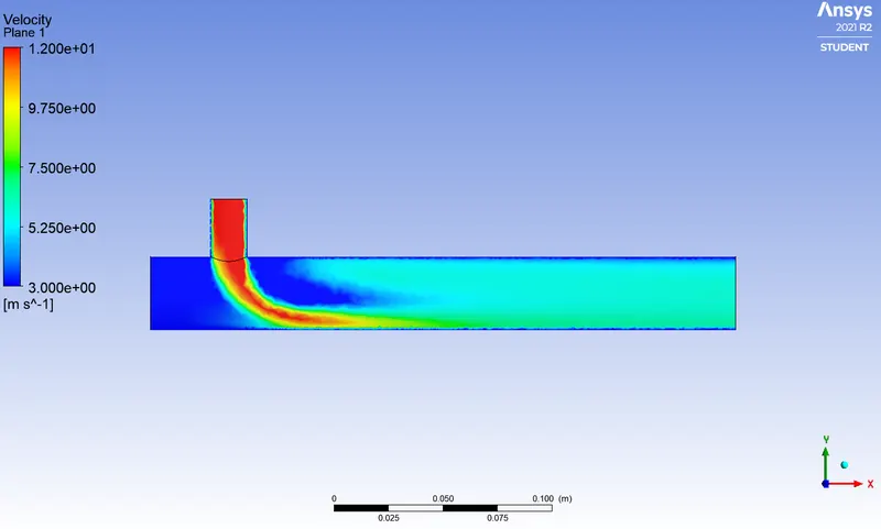
The post processing results are as follows :

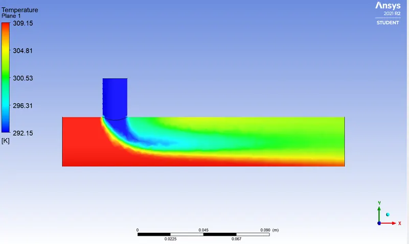
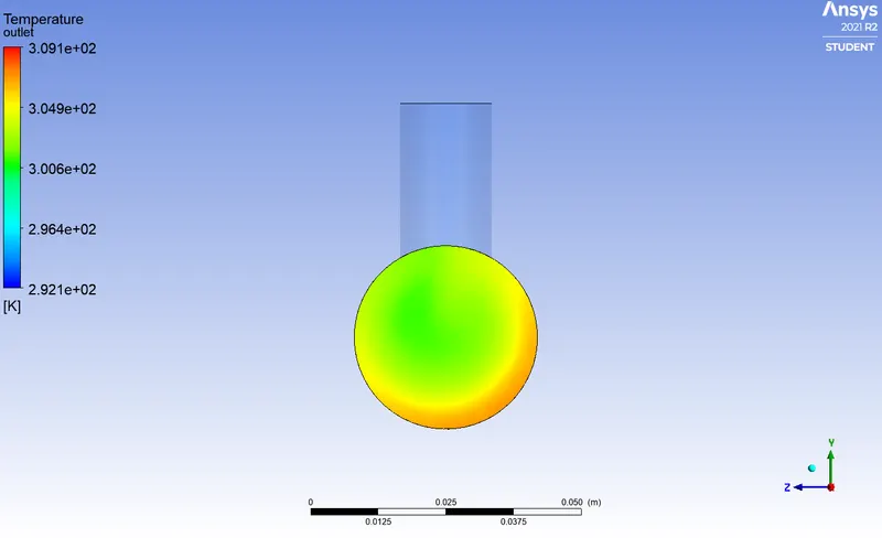
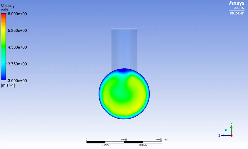
we can see that the temperature is still not mixed with the cool air as it moves out. The velocity profile is as follows :

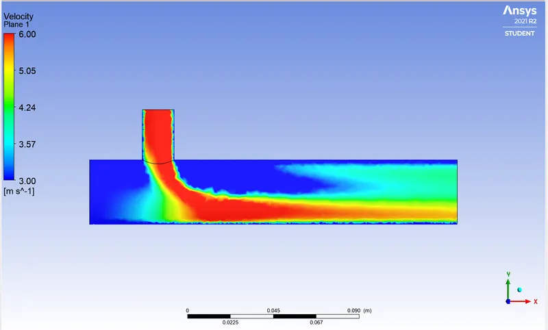
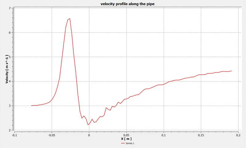
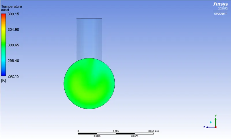
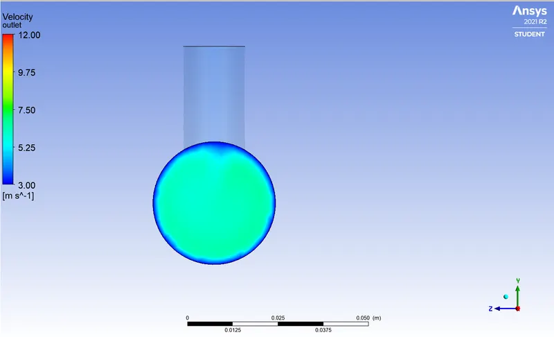
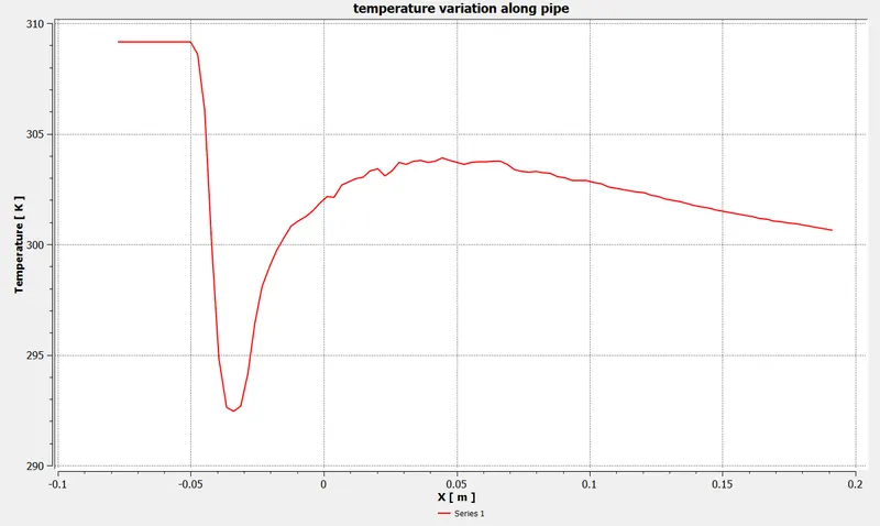
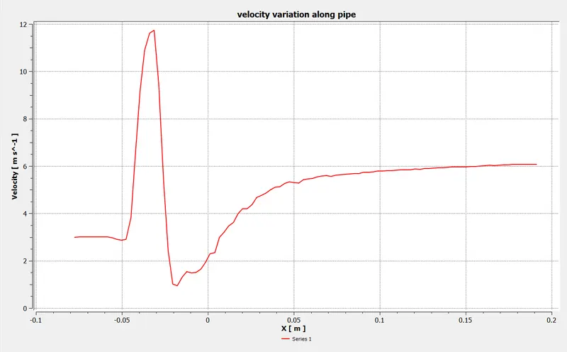
the temperature and velocity profile across outlet are as follows :

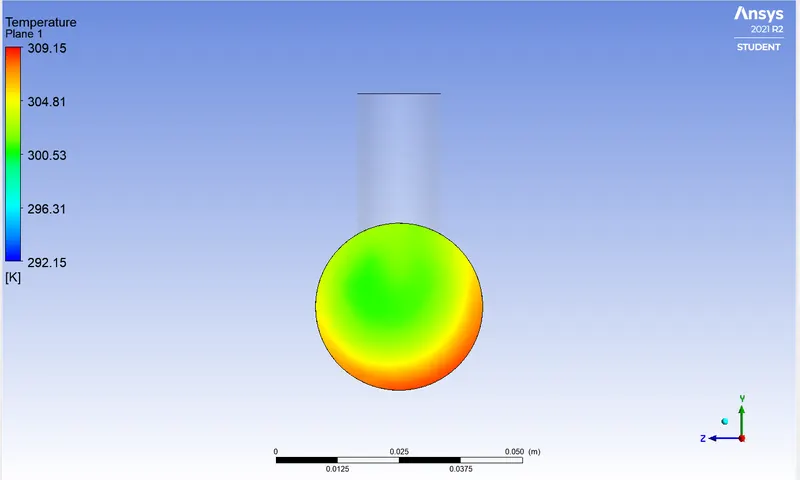
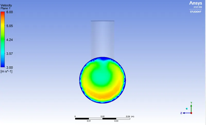
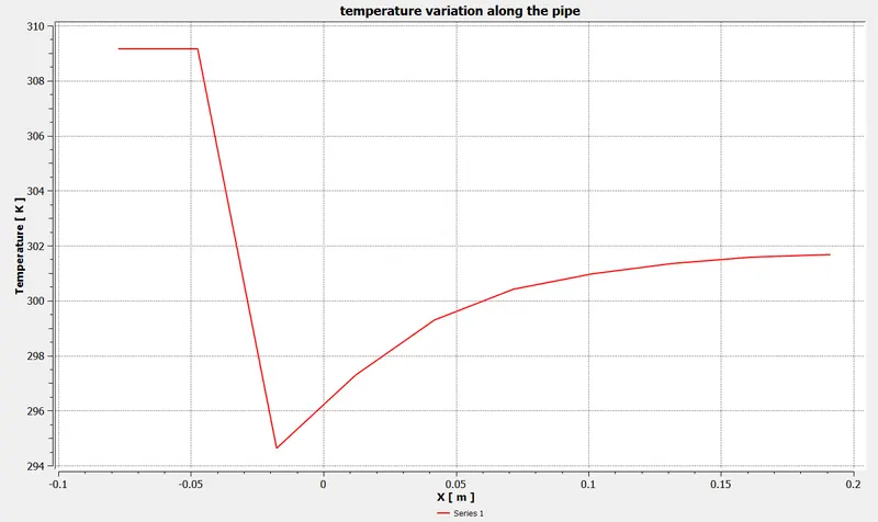
the line plot for the same is follows :

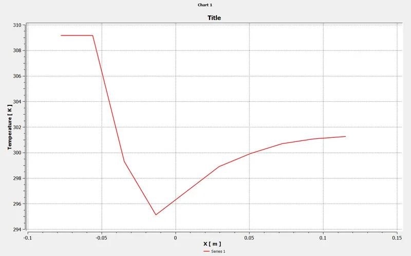
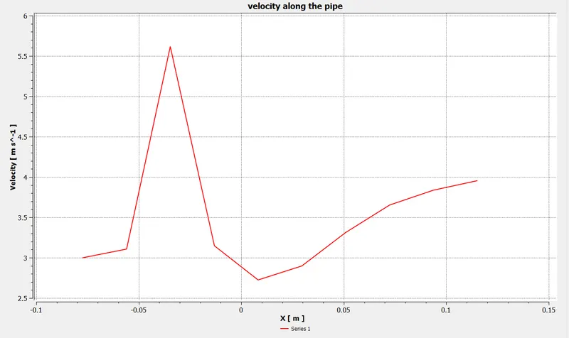
now, Case 2 : where the momentum ratio is 2. Here we have used k- omega model for solving the equations :

inlet velocity along x-axis = 3m/s and along y-axis = 6m/s

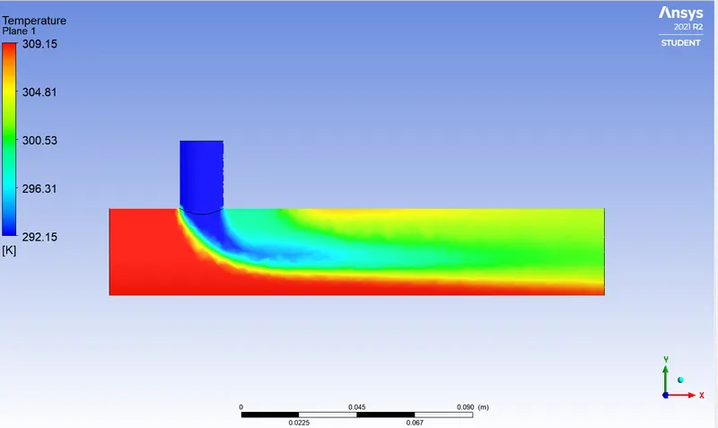
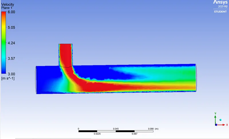
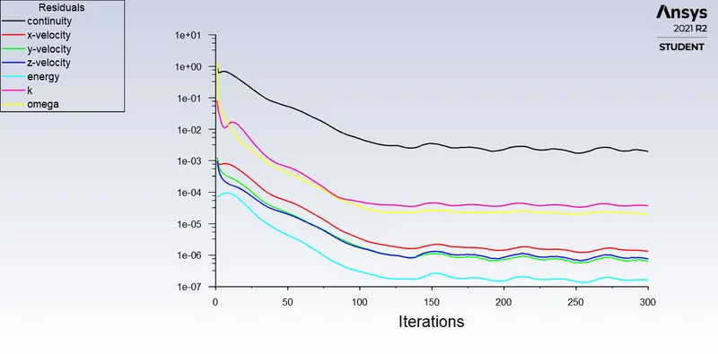
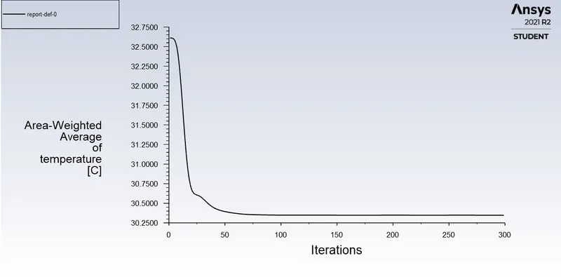
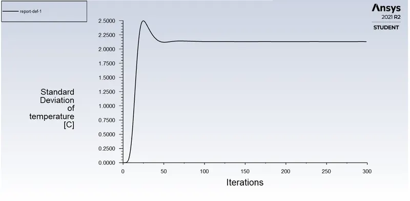
The `k-epsilon` model is able to converge at lower no. of iterations when we consider the default value for mesh element size. Hence moving forward we will be solving for further cases in `k-epsilon` model.

Case 3 :

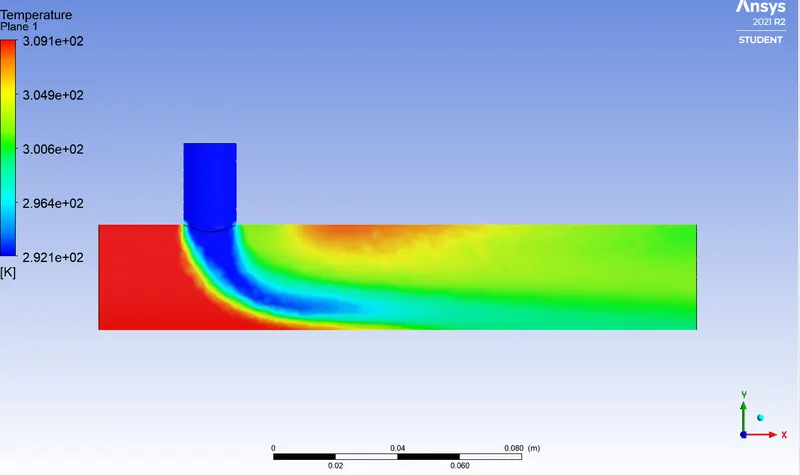
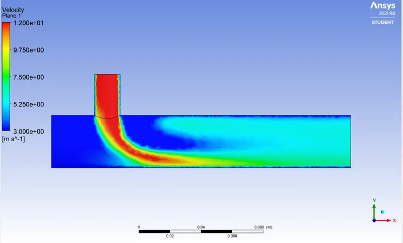
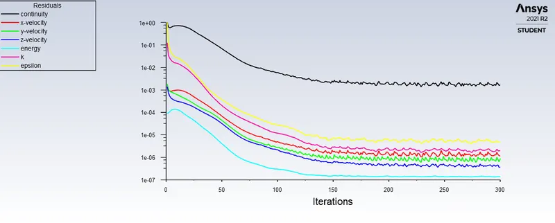
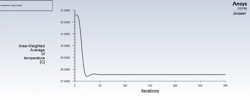
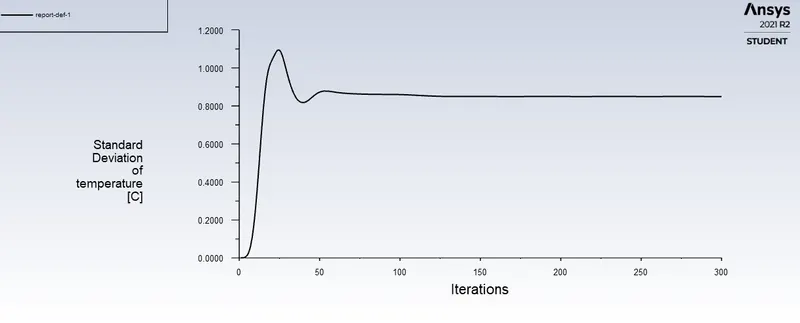
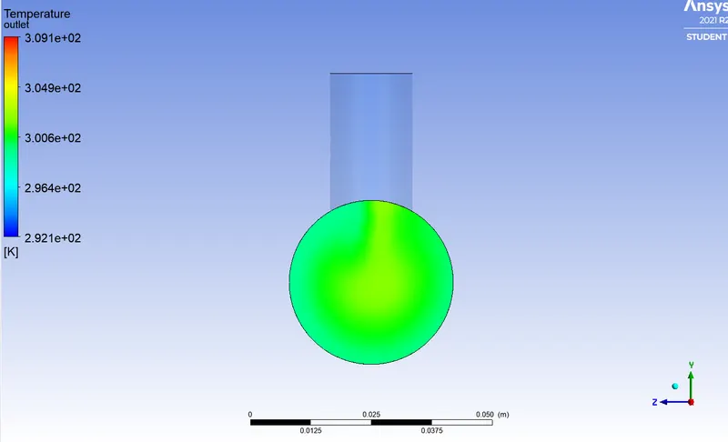
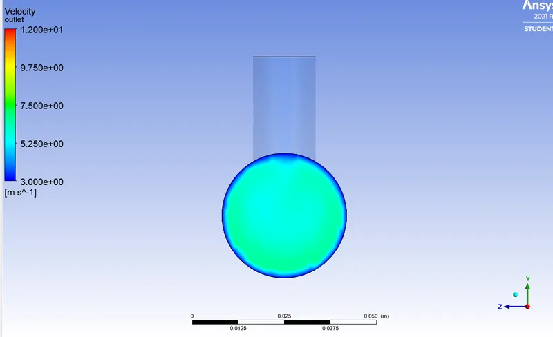
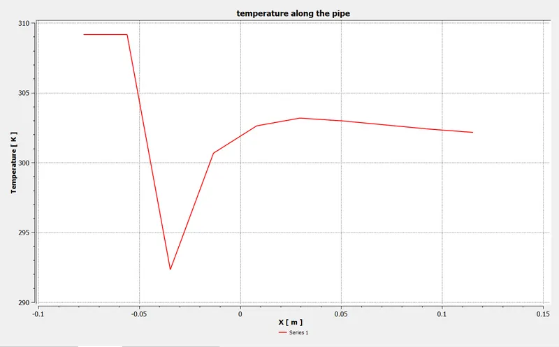
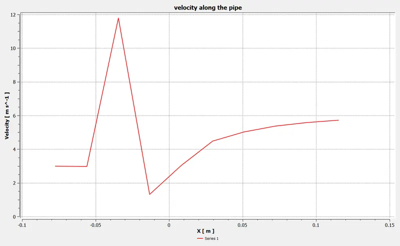
Here the inlet-y velocity is 12 m/s . the momentum ratio is 4.

the results are as follows :

Case 4 :

Here we use a slightly longer pipe to simulate the results and see if if affects the temperature at the outlet.

we start with the momentum ratio of 2 and then for 4.

The simulation results are as follows :

we can see from the simulation at this configuration we get a proper mix of both the temperature at the outlet and we get relatively cooler air than the air at inlet-x.

Case 5 :

here the inlet-y velocity is 12 m/s and the longer pipe is used a geometry.

Case Setup	Cell count	Standard deviation (outlet temperature) degree celcius	Average outlet temperature (degree celcius)	Number of iterations for convergence	Solver used
Short pipe with flow momentum ratio of 2	104931	2.03655	30.26	125	k-epsilon solver
Short pipe with flow momentum ratio of 2	104931	2.0365	30.262	150	k-omega solver
Short pipe with flow momentum ratio of 4	104931	0.8491	27.54	125	k-epsilon solver
Long pipe with flow momentum ratio of 2	138811	1.6555	30.3525	125	k-epsilon solver
Long pipe with flow momentum ratio of 4	138811	0.6401	27.4981	125	k-epsilon solver

Conclusion :

Increasing the air flow velocity has shown a noticeable difference in the mixing phase of the 2 different velocity air flows. But increasing the length has not contributed significantly in cooling.

Grid Dependency test :

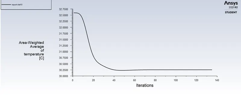
First I tried the results with the base line mesh where default value of mesh elements is selected by the system and checked the value of area weighted average and standard deviation for temperature. The results are as follows :

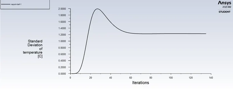
Now we fine the mesh elements to 1.9e-4 and check the results :

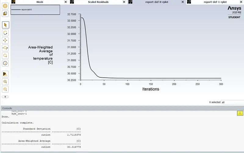
we can see that the value for area weighted average temperature for outlet is almost same for all the cases with similar physical properties.

Hence making the mesh even finer is not putting any additional refinements in the data.

====================================== end =============================================