MATLAB Program - Linear Convection

Aim: To obtain solution of one dimension linear convection equation.

Objective:

• Obtain numerical solution of linear convection equation by first order finite differencing schemes.
• Obtaining plots for the same; compare the initial velocity profile and the final velocity profile.
• Note the variations by keeping
  • time step constant and varying the grid size.
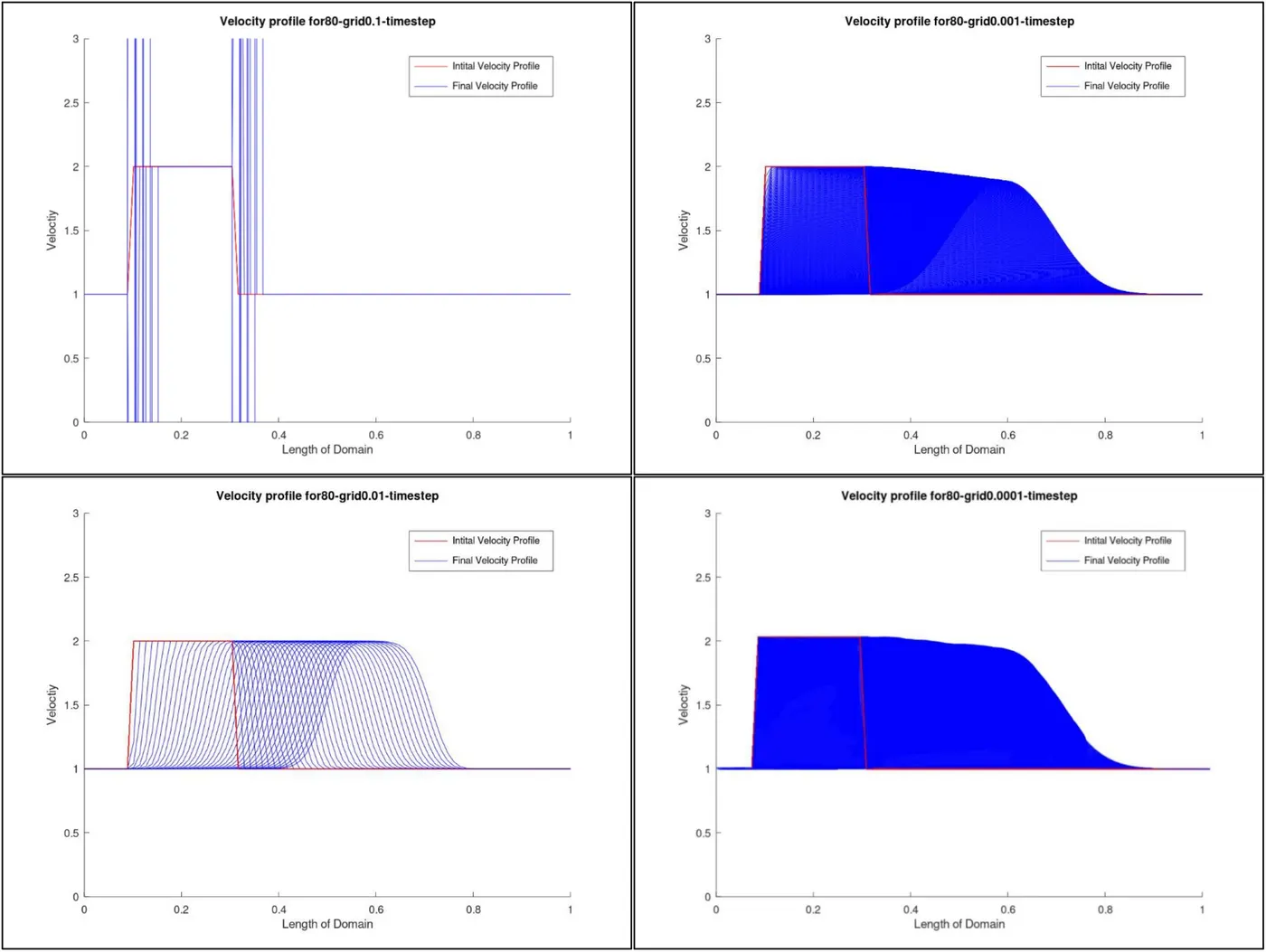
  • grid size constant and varying time step.

Thus, check the stability of obtained solution.

Theory:

Numerical Discretization:

In applied mathematics, discretization is the process of transferring continuous functions, models, variables, and equations into discrete counterparts. This process is usually carried out as a first step towards making them suitable for evaluation and/or implemetation in computing techniques.

In this program, we'll use forward differencing scheme in time and backward differencing in space to obtain the velocity profile.

Linear Convection:

After neglecting the diffusive terms and assuming one dimensional flow in the Navier-Stokes equation, we arrive at,

`(delu)/(delt) + c(delu)/(delx) = 0`

The above equation describes the 1-D linear convection, where, the first term is the local term and the second term denotes the convective part.

In this program, we'll solve the above equation by aforementioned schemes, with the initial conditions of a square wave and constant boundary conditions.

Code:

The program is written in MATLAB.

1. Main Script

%Linear Convection -Varying Grid
clear all
close all
clc

% Inputs for the linear convention
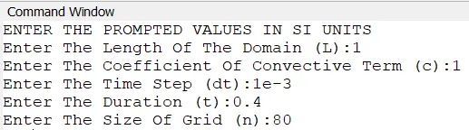
printf("ENTER THE PROMPTED VALUES IN SI UNITSn")
L = input('Enter The Length Of The Domain (L):');
c = input('Enter The Coefficient Of Convective Term (c):');
dt = input('Enter The Time Step (dt):');
t_end = input('Enter The Duration (t):');
nt = (0.01:dt:t_end); 
n = input('Enter The Size Of Grid (n):');
%calculation

x = linspace(0,L,n);
dx =x(2)-x(1);
%dx = L/(n-1)

% Define the start and end positions for the square wave
x_start = 0.1;
x_end = 0.3;
 
% n_start =f(x_start)
% n_end = f(x_end)

n_start = func_start(x,x_start); %Function to calculate n_start
n_stop =  func_end(x,x_end);   %Function to calculate n_stop

% Intialize arrays and apply boundary conditions
u = ones(1,n);
u(n_start:n_stop)= 2; %Velocity profile = 2m/s between 0.1 and 0.3

%Boundary Conditions
u(1) = 1;
uold = u;
u_initial = u;

ct = 1;
%Time loop
for k =1:length(nt)
  % space loop
  % du/dt = -c*du/dx
  % du/dx - FDS,CDS, BDS, skewed schemes
  for i =2:n
    u(i) = uold(i)-(c*dt/dx)*(uold(i) - uold(i-1)); % FDS for space loop
  end
  % Update old velocitites
  uold = u;
  
  %Plotting the velocties 
  figure(1)
  plot(x, u_initial,'r',x,u,'b')
  axis ([0 1 0 3],"manual")
  xlabel('Length of Domain')
  ylabel('Veloctiy')
  legend('Intital Velocity Profile','Final Velocity Profile')
  caption = ['Velocity profile for',num2str(n),'-grid',num2str(dt),'-timestep'];
  title(caption)
  text = [caption,'-',num2str(ct),'.png'];
  saveas(1,text)
  ct = ct+1;
  
  figure(2)
  hold on
  plot(x, u_initial,'r')
  plot(x,u,'b');
  axis ([0 1 0 3],"manual")
  xlabel('Length of Domain');
  ylabel('Veloctiy');
  legend('Intital Velocity Profile','Final Velocity Profile');
  caption = ['Velocity profile for',num2str(n),'-grid',num2str(dt),'-timestep'];
  title(caption);
end
%Saving the final plot
text = ['Velocity profile for',num2str(n),'grid-',num2str(dt),'timestep','.png']; 
saveas(2,text);

2. function to caculate the start of square wave

function out = func_start(x,x_start)
  for i = 1:length(x);
    Z(i) = abs(x_start-x(i)); %Z is the difference
  endfor
  [num,out] = min(Z);
endfunction

3. function to calculate the end of sqaure wave

function out = func_end(x,x_end)
  for i = 1:length(x);
    Z(i) = abs(x_end-x(i)); %Z is the difference
  endfor
  [num,out] = min(Z);
endfunction

Working of Code:

1. The Program begins with clear all, close all, clc; which means clear the workspace, close all figure windows and clear the command line respectively.

2. Inputs, like the domain length, time step, time duration,etc. are prompted to be entered by the user. Once the entries are registered, further calculations are done on the basis of these inputs.

3. The domain is divided into the number of parts specified by the grid size. Later on, the initial condition of square wave, i.e. the initial position is stated in x_start and x_end. These are fed into a function, where, the propagation of this wave is caculated and the values are provided to n_start and n_stop.

4. The initial values of the flow velocity and wave velocity is also defined. Based on this, the loops are run on linear convection equation for calculating the velocity profile.

5. A nested for loop is used here. The outer loop is run using time steps and the inner loop, calculates the velocity is the space loop. These loops are successively iterated to simulate the square wave to appear as if it is moving.

6. The profile is plotted within the loop, so that, each frame is captured ( and not only the final profile). The embelished plots (with suitable titles and labels) are saved. This completes the program.

Outputs:

Varying Grid Size:

1. Grid-20 Time Step - 1e-2

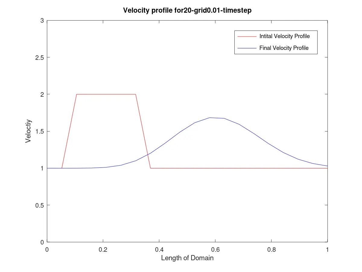
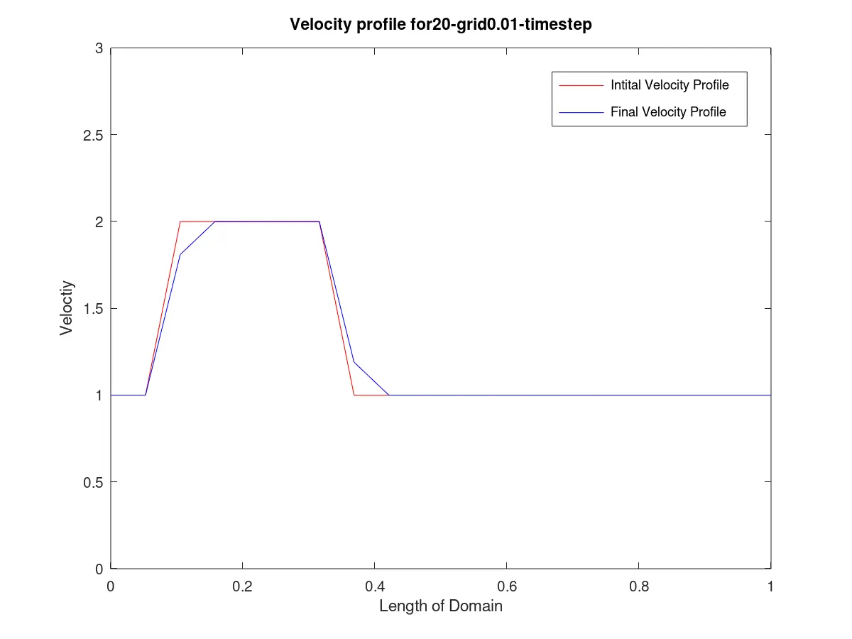
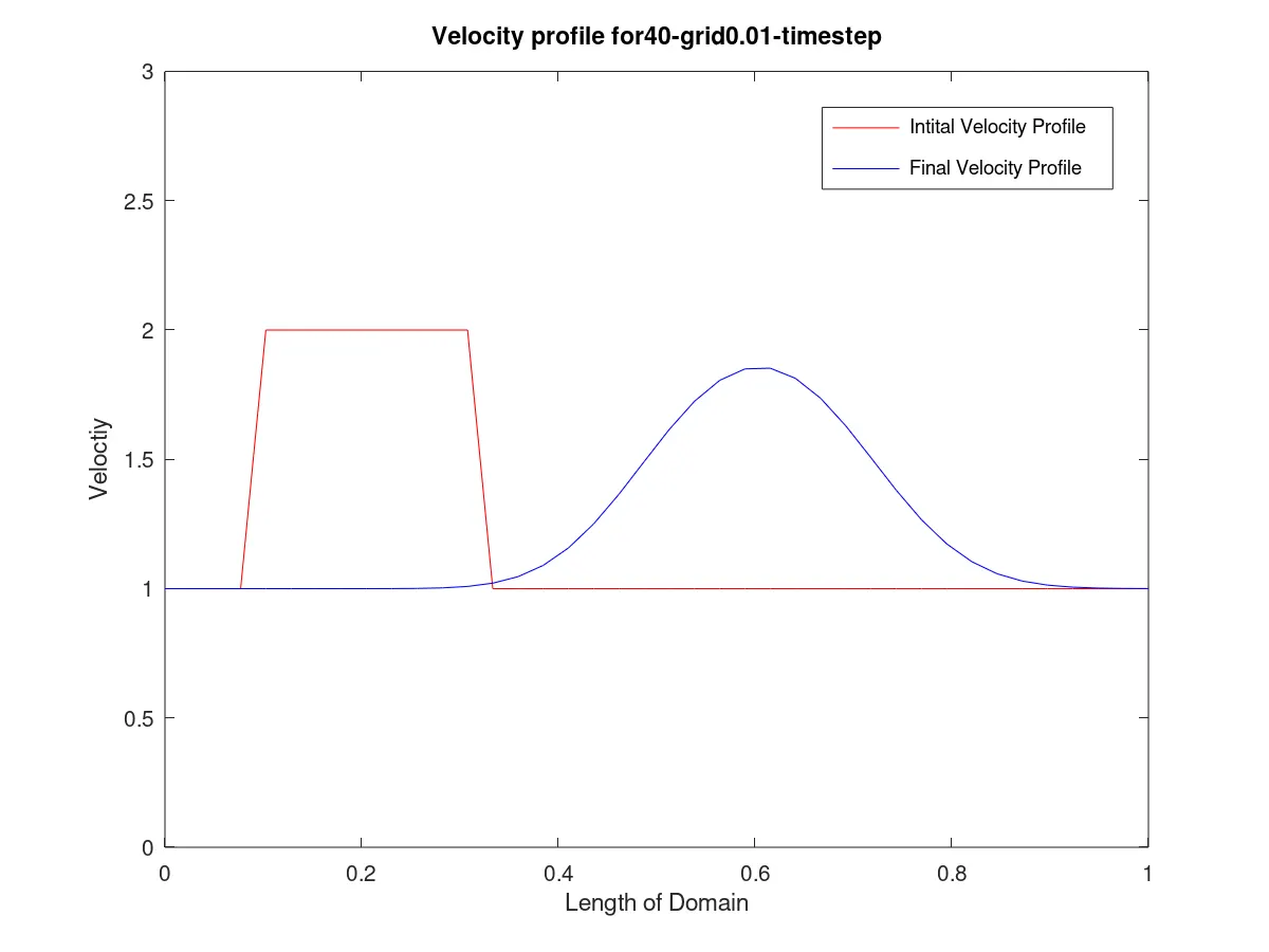
2. Grid-40 Time step - 1e-2

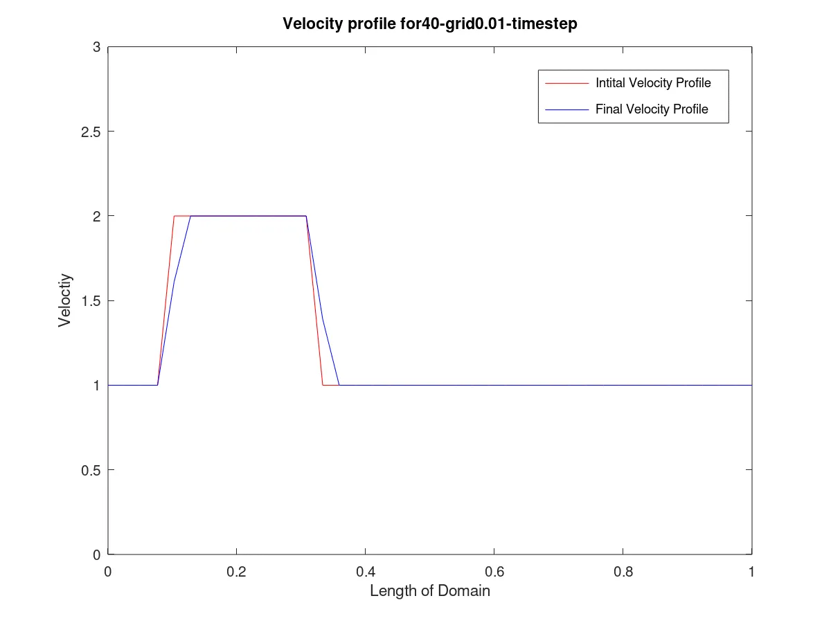
3. Grid-80 Time step - 1e-2

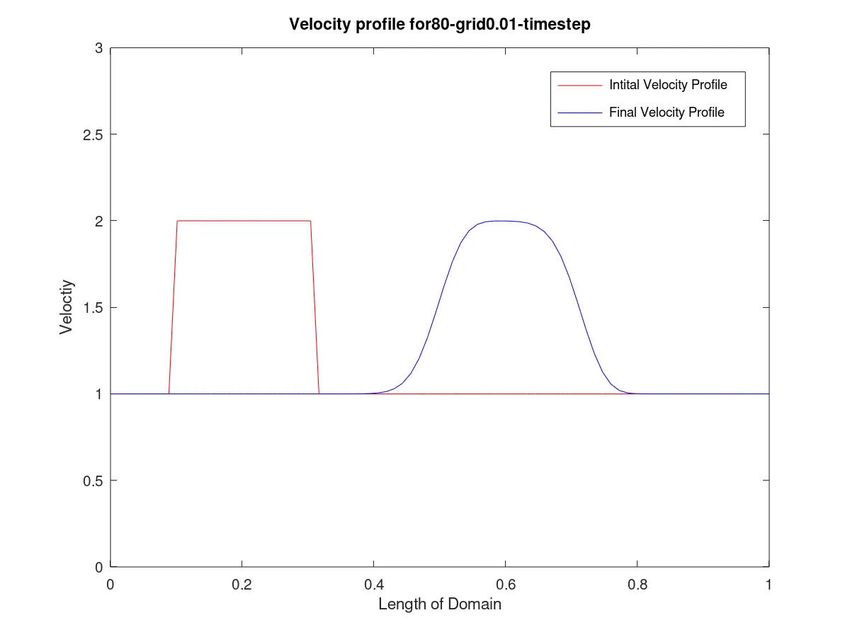
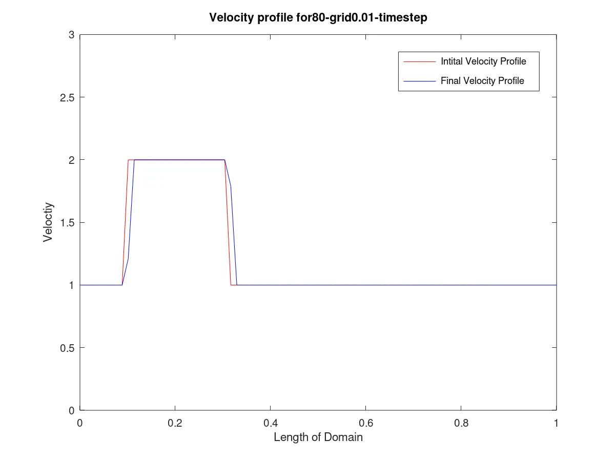
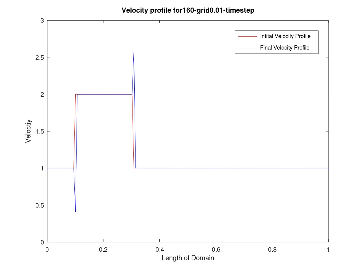
4. Grid-160 Time step - 1e-2

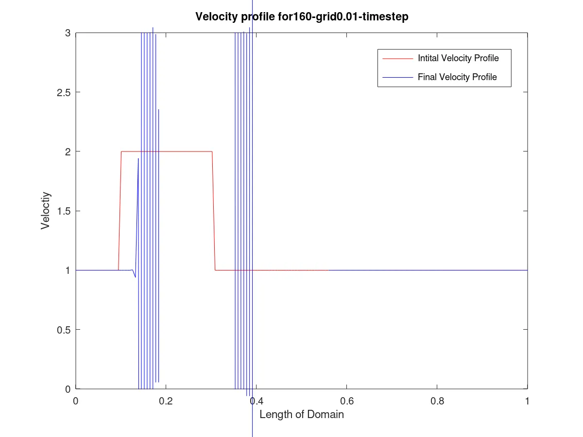
Varying Time-Step:

Velocity profiles at t=0.4s, grid size - 80

Result/Conclusion:

• A solution is obtained and stability is studied by varying the grid size.
• It is evident from above plots that
  • with increase in grid size, the solution becomes smoother, and the convection is easier to notice. But tremendously high grid size brings in wobbling and oscillations, thus solution is known to get unstable.
  • keeping the time step too large can increase the error to an extent that the solution gets spoiled, and having a too small step size cannot give much inference and rather become resource extensive. Hence, an optimum time step leads to a beautiful result.
• The square wave isn't maintained because of artificial diffusion induced by the errors of forward differencing scheme.
• The square is being convected by a constant linear velocity `c`, hence wave propagates towards right.

References:

• Introduction to CFD using MATLAB and OpenFOAM - Course provided by Skill Lync.
• GNU Octave
• Higher Engineering Mathematics - BS Grewal
• Fluid Mechanics - FM White