Linear Convection for varying number of time steps using MATLAB

Aim : To demonstrate the linear convection equation in graphical format with varying number of time steps and keeping the no. of nodes constant.

Procedure : The linear convection equation is solved using time marching procedure. First we discretize the equation with first order forward difference method for the first part of the equation and first order backward difference method for the second half of the equation.

the equation is given as : `(delu)/(delt) + c*(delu)/(delx) = 0`

so `(delu)/(delt)` is discretized by forward difference method and `(delu)/(delx)` is discretized by using backward difference method.

since we are observing the effect of varying no. of time steps , we consider the range of dt = [1e-4, 1e-3, 1e-2, and 1e-1].

the length of the domain is given as 1 metre.

constant convection co-efficient = c = 1 m/s.

simulation run time :t = 0.4 seconds

we create an array of x values on graph and plot the velocity profile.

the initial condition for the velocity profile is 1 m/s and a step function of 2m/s is expected between x = 0.1 and 0.3.

here explicit method is used to discretize the PDE.

the expression is given as follows : `(delu)/(delt) + c*(delu)/(delx) = 0`

after applying forward difference first order derivative on `(delu)/(delt)`term and backward difference first order derivative on `(delu)/(delx)` , we get

`therefore (u_2^(n+1) -u_2^n)/(delt) + c*[(u_2^n - u_1^n)/(delx)] = 0`

`therefore u_2^(n+1) = u_2^n - c*(delt)/(delx)[u_2^n - u_1^n]`

Suppose we consider this equation for n = 1 time step and node i = 2, the initial conditions are known hence we dont compute the values for it.

`u_2^2 = u_2^1 - c*(delt)/(delx)*[u_2^1 - u_1^1]`

since, `u_2^1 and u_2^2= 1 m/s` as per the initial condition, we get `

`u_2^2 = 1 - c*(delt)/(delx)*[1-1]`

`u_2^2 = 1`

similarly, at node = 3 , `u_3^2 = u_3^1 - c*(delt)/(delx)[u_3^1 - u_2^1] = 1`

when we rewrite the equation as :

`(u_i^(n+1) - u_i^(n))/(delt) = -c* [(u_i^(n) - u_(i-1)^(n))/(delx)]`

since the right hand side terms are known , we consider this equation as explicit method of integration.

the code which solves for n = 80 and for varying time steps is given as follows :

clear all
close all
clc

n = 80
L = 1;
dt = [1e-4 1e-3 1e-2 1e-1]
t = 0.4;
x = linspace(0,L,n);
dx = L/(n-1);
t = 0.4;
c = 1;

%nt = t/dt;

for i = 1:length(dt)
    nt = t/dt(i);
    
    [u(i,:),u_initial] = timestep_1(n,c,dx,dt(i));
end
   
figure(1)
plot(x,u_initial,'linewidth',2)
hold on
plot(x,u(1,:),'linewidth',2)
plot(x,u(2,:),'linewidth',2)
plot(x,u(3,:),'linewidth',2)
plot(x,u(4,:),'linewidth',2)
grid on
xlabel('x axis')
ylabel('velocity')
legend('initial','1e-4','1e-3','1e-2','1e-1')
axis([0 1 0 3])
    
    
  

###############################

u(i,;) is employed in this code ,since we need to utilise the rows for every iteration of u as it varies from 1 to 4.

the function is called in the main code to compute u at different values of dt

the function for given code is as follows :

function [u,u_initial] = timestep_1(n,c,dx,dt)
L = 1;
c = 1; 

n = 80
t = 0.4  
% calculations
x = linspace(0,L,n);
%R = round(find(x == 0.1))
%Y = round(find(x == 0.3))
%dx = x(2) - x(1)
dx = L/(n-1)

% define the start and end positions for the square wave
        
%n_start = 0.1
%n_stop = 0.3
x_start = round((0.1/dx))+1;
x_stop = round((0.3/dx))+1;



% initialize arrays and apply boundary conditions
u = ones(1,n);
u(x_start:x_stop) = 2;
% BC 
u(1) = 1;
uold = u;
u_initial = u;

nt =  t/dt
% timp loop
    for k = 1:nt

    % space loop
    for i = 2:n
    u(i) = uold(i) - (c*dt/dx)*(uold(i) - uold(i-1));
    
    end
    
    %update old velocities
    uold = u;
    end
    
end
    
    
    

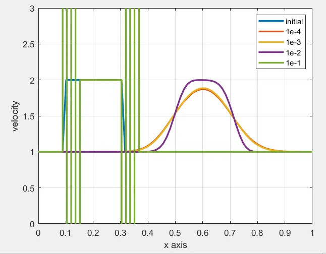
the graph results are as follows :

CFL criteria :

The CFL criteria is generally given as `c*(delu)/(delx)` `< 1`

`c*(delu)/(delx)` is called as courant no.

when the courant no. meets the criteria of CFL ,we get the stable solution. Previously we saw the change of velocity as we calculated it for varying no. of nodes. It appears that the variation of time steps also contributes to the stability.

As per the code we change the value of dt from 1e-4, 1e-3, 1e-2, and 1e-1 . As we increase the value of time step the solution gets stable but at dt = 1e-1 the courant no become more than 1 and hence we the solution blowed up.

Therefore, what we can conclude is not only there is a limit to decreasing dx for getting an exact solution but also there is a limit to increasing time step size for obtaining an accurate result. Putting it all together, we can say that, courant no. has a range in which we can get stable results but outside that range our solution blows up. This also known as stability criteria.

Also to note, that the diffusion term was not introduced in the equation but still we get to see the effect in our graph. That is because when we discretize the PDE we had ignored the higher order terms which are contributing to the diffusion in equation.

============================= end ===============================