Linear Convection for varying number of nodes

Aim : To demonstrate the linear convection equation in graphical format with varying number of nodes.

Procedure : The linear convection equation is solved using time marching procedure. First we discretize the equation with first order forward difference method for the first part of the equation and first order backward difference method for the second half of the equation.

the equation is given as : `(delu)/(delt) + c*(delu)/(delx) = 0`

so `(delu)/(delt)` is discretized by forward difference method and `(delu)/(delx)` is discretized by using backward difference method.

since we are observing the effect of varying values of no. of nodes. we consider them as [20,40,80,160].

the length of the domain is given as 1 metre.

constant convection co-efficient = c = 1 m/s.

time step = dt = 0.01

simulation run time :t = 0.4 seconds

we create an array of x values on graph and plot the velocity profile.

the initial condition for the velocity profile is 1 m/s and a step function of 2m/s is expected between x = 0.1 and 0.3.

here explicit method is used to discretize the PDE.

the expression is given as follows : `(delu)/(delt) + c*(delu)/(delx) = 0`

after applying forward difference first order derivative on `(delu)/(delt)`term and backward difference first order derivative on `(delu)/(delx)` , we get

`therefore (u_2^(n+1) -u_2^n)/(delt) + c*[(u_2^n - u_1^n)/(delx)] = 0`

`therefore u_2^(n+1) = u_2^n - c*(delt)/(delx)[u_2^n - u_1^n]`

Suppose we consider this equation for n = 1 time step and node i = 2, the initial conditions are known hence we dont compute the values for it.

`u_2^2 = u_2^1 - c*(delt)/(delx)*[u_2^1 - u_1^1]`

since, `u_2^1 and u_2^2= 1 m/s` as per the initial condition, we get `

`u_2^2 = 1 - c*(delt)/(delx)*[1-1]`

`u_2^2 = 1`

similarly, at node = 3 , `u_3^2 = u_3^1 - c*(delt)/(delx)[u_3^1 - u_2^1] = 1`

when we rewrite the equation as :

`(u_i^(n+1) - u_i^(n))/(delt) = -c* [(u_i^(n) - u_(i-1)^(n))/(delx)]`

since the right hand side terms are known , we consider this equation as explicit method of integration.

implicit method is given as : `(u_i^(n+1) - u_i^(n))/(delt) = -c* [(u_i^(n+1) - u_(i-1)^(n+1))/(delx)]`

for time step = 1, we get

`(u_2^2 - u_2^1)/(delt) = -c*[(u_2^2 - u_1^2)/(delx)]`

consider k = `-c*(delt)/(delx)`we get

`(u_2^2 - u_2^1) = k*(u_2^2 - u_1^2)`

`therefore u_2^2 - k*u_2^2 + k*u_1^2 = u_2^1` at node = 2

`therefore u_3^2 - k*u_3^2 + k*u_2^2 = u_3^1` at node = 3

`u_4^2 - k*u_4^2 + k*u_3^2 = u_4^1` at node = 4

since the right hand side terms are not known here,

we have 4 equations for different nodes, representing it in matrix is as follows :

`[[1,0,0,0],[k,1-k,0,0],[0,k,1-k,0],[0,0,k,1-k]]` * `[[u_1^2],[u_2^2],[u_3^2],[u_4^2]]` = `[[1],[u_2^1],[u_3^1],[u_4^1]]`

hence we can find the velocity profile for the next time step with this matrix.

## For this challenge , we will use explicit method to solve the linear convection equation :

the code is as follows :

clear all
close all
clc

% inputs for the linear convection problem

n = [20 40 80 160];
ct = 1
for j = 1:length(n)
    
L = 1;
c = 1; 
dt = 1e-2

    
% calculations
x = linspace(0,L,n(j));
%R = round(find(x == 0.1))
%Y = round(find(x == 0.3))
%dx = x(2) - x(1)
dx = L/(n(j)-1)

% define the start and end positions for the square wave
        
%n_start = 0.1
%n_stop = 0.3
x_start = round((0.1/dx))+1;
x_stop = round((0.3/dx))+1;



% initialize arrays and apply boundary conditions
u = ones(1,n(j));
u(x_start:x_stop) = 2;
% BC 
u(1) = 1;
uold = u;
u_initial = u;

% plot tp
%plot(x,u)

nt = 40  % t/dt = 0.4/0.01
% timp loop
    for k = 1:nt
    
    % space loop
    for i = 2:n(j)
    u(i) = uold(i) - (c*dt/dx)*(uold(i) - uold(i-1));
    
    end

    %update old velocities
    uold = u;
    
    figure(j)
    plot(x,u_initial,'r')
    hold on
    plot(x,u,'b')
    hold off
    grid on
    xlabel('x axis')
    ylabel('velocity')
    legend('initial velocity','final velocity')
    axis([0 1 0 3])
    pause(0.03)
    M(ct)=getframe(gcf);
    ct = ct + 1
    end
    
end
    movie(M)
    videofile = VideoWriter('linear_convection.avi','Uncompressed AVI');
    open(videofile)
    writeVideo(videofile,M)
    close(videofile)

'find' command could have been used but it holds good when we are dealing with integers.

the plots are as follows :

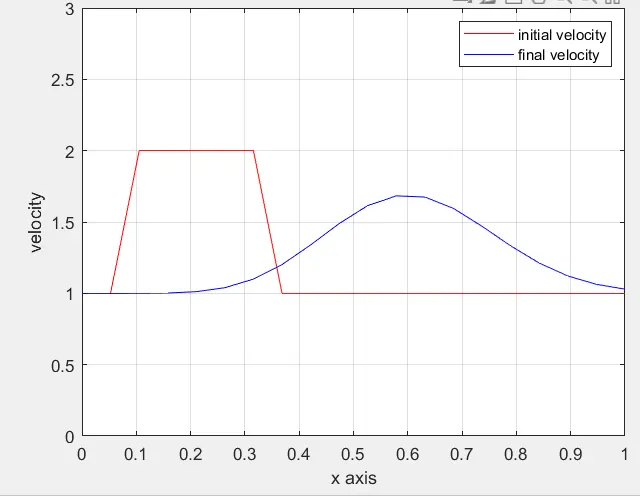
plot with n = 20

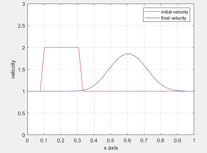
plot with n = 40

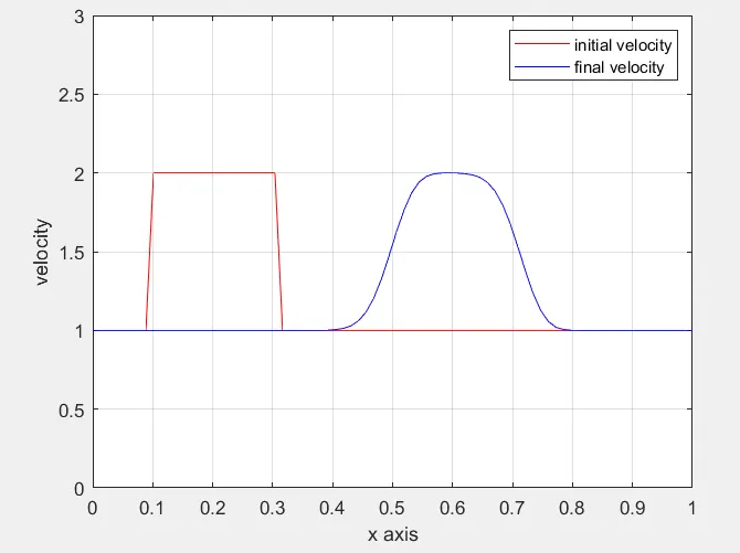
plot with n = 80

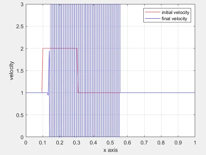
plot with n = 160

the animation file for all the varying no. of nodes is as follows :

Conclusion : From the graphs generated after we vary the number of nodes in this equation, we observe different results.

With respect to the initial step function we can see that the peak of the curve starts to decline and we encounter a phenomenon called as artificial diffusion. It was not introduced in the code , still we get this diffusion.

This diffusion is dependent on the factor called as courant number = `c*(delu)/(delx)`

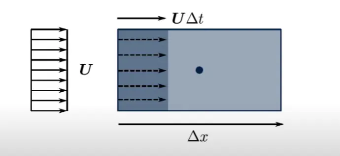
Courant No. = Courant No. is the ratio of fluid moving across the cell to the size of the cell. Suppose a fluid element is subjected to a velocity as u ( as given in above figure) . Over a time step `delt`, the flow moves a distance `u*delt` across the cell with distance `delx`. So courant no. is given as the ratio of these two lengths or we can say the fraction of the cell that move across in a time step.

graph for when n = 101 :

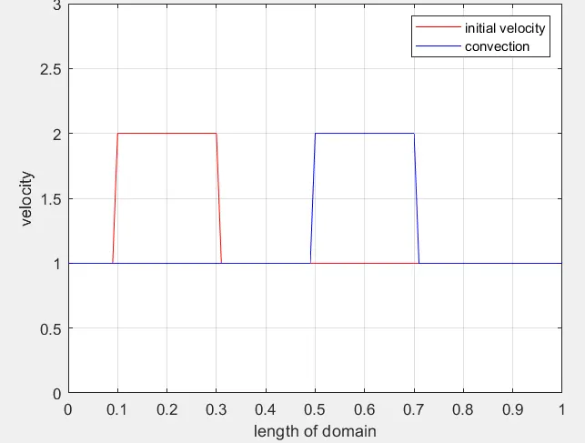
for n = 20,40,80 the graph seems to be stable. But when reaches n = more than 101, we observe that the solution gets blown up. At n = 101 the convection as no losses. From this we can state that when the courant number is less that 1, then there will be artificial diffusion but the solution would be stable. When the courant no. is more than 1, the solution becomes unstable. But when it is 1, that means when n = 101, the solution is not only stable but the diffusion is negligible or zero.

===========================End===========================