Independent Research Project
PROJECT REPORT
INDEPENDENT RESEARCH PROJECT
MOHR'S CIRCLES
OBJECTIVE :
The aim of this project is to construct 2D and 3D Mohr circle diagram for a specefic loading condition and to calculate principal stresses developed over the specimen using PYTHON codes.
THEORY :
2D MOHR CIRCLE
The 2-D stresses, so called plane stress problem, are usually given by the three stress components sx , sy , and txy , which consist in a two-by-two symmetric matrix (stress tensor):
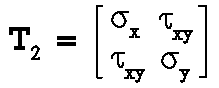
What people usually are interested in more are the two prinicipal stresses s1 and s2 , which are the two eigenvalues of the two-by-two symmetric matrix of Eqn (1), and the maximum shear stress tmax , which can be calculated from s1 and s2 . Now, see the Fig. 1 below, which represents that a state of plane stress exists at point O and that it is defined by the stress components sx , sy , and txy associated with the left element in the Fig. 1. We propose to determine the stress components sxq , syq , and txyq associated with the right element after it has been rotated through an angle q about the z axis.
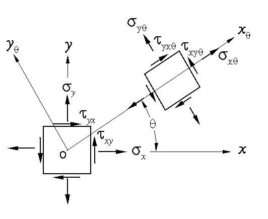
Then, we have the following relationship:
and
Equivalently, the above two equations can be rewritten as follows:
and
The expression for the normal stress syq may be obtained by replacing the q in the relation for sxq in Eqn. 3 by q + 90o , it turns out to be
From the relations for sxq and syq , one obtains the circle equation:
where
This circle is with radius R2m and centered at C = (save , 0) if let s = sxq and t = -txyq as shown in Fig. 2 below - that is right the Mohr's Circle for plane stress problem or 2-D stress problem!
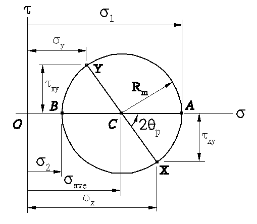
In fact, Eqns. 4 and 5 are the parametric equations for the Mohr's circle! In Fig. 2, one reads that the point
which corresponds to the point at which q = 0 and the point
which corresponds to the point at which q = qp that gives the principal stress s1 ! Note that
and the point
which corresponds to the point at which q = 90o and the point
which corresponds to the point at which q = qp + 90o that gives the principal stress s2 ! To this end, one can pick the maxium normal stressess as
Besides, finally one can also read the maxium shear stress as
which corresponds to the apex of the Mohr's circle at which q = qp + 45o !
Mohr's Circles for 3-D Stress Analysis
The 3-D stresses, so called spatial stress problem, are usually given by the six stress components sx , sy , sz , txy , tyz , and tzx , (see Fig. 3) which consist in a three-by-three symmetric matrix (stress tensor):
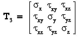
What people usually are interested in more are the three prinicipal stresses s1 , s2 , and s3 , which are eigenvalues of the three-by-three symmetric matrix of Eqn (16) , and the three maximum shear stresses tmax1 , tmax2 , and tmax3 , which can be calculated from s1 , s2 , and s3 .
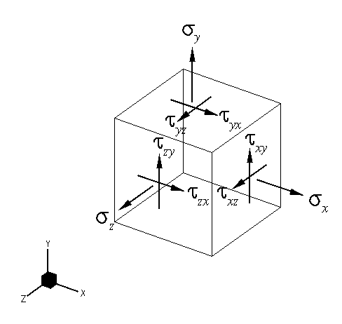
Imagine that there is a plane cut through the cube in Fig. 3 , and the unit normal vector n of the cut plane has the direction cosines vx , vy , and vz , that is
then the normal stress on this plane can be represented by
There exist three sets of direction cosines, n1, n2, and n3 - the three principal axes, which make sn achieve extreme values s1 , s2 , and s3 - the three principal stresses, and on the corresponding cut planes, the shear stresses vanish! The problem of finding the principal stresses and their associated axes is equivalent to finding the eigenvalues and eigenvectors of the following problem:
The three eigenvalues of Eqn (19) are the roots of the following characteristic polynomial equation:
where
In fact, the coefficients A, B, and C in Eqn (20) are invariants as long as the stress state is prescribed(see e.g. Ref. 2) . Therefore, if the three roots of Eqn (20) are s1, s2 , and s3 , one has the following equations:
Numerically, one can always find one of the three roots of Eqn (20) , e.g. s1 , using line search algorithm, e.g. bisection algorithm. Then combining Eqns (24)and (25), one obtains a simple quadratic equations and therefore obtains two other roots of Eqn (20), e.g. s2 and s3 . To this end, one can re-order the three roots and obtains the three principal stresses, e.g.
Now, substituting s1 , s2 , or s3 into Eqn (19), one can obtains the corresponding principal axes n1, n2, or n3 , respectively.
Similar to Fig. 3, one can imagine a cube with their faces normal to n1, n2, or n3 . For example, one can do so in Fig. 3 by replacing the axes X,Y, and Z with n1, n2, and n3 , respectively, replacing the normal stresses sx , sy , and sz with the principal stresses s1 , s2 , and s3 , respectively, and removing the shear stresses txy , tyz , and tzx .
Now, pay attention the new cube with axes n1, n2, and n3 . Let the cube be rotated about the axis n3 , then the corresponding transformation of stress may be analyzed by means of Mohr's circle as if it were a transformation of plane stress. Indeed, the shear stresses excerted on the faces normal to the n3 axis remain equal to zero, and the normal stress s3 is perpendicular to the plane spanned by n1 and n2 in which the transformation takes place and thus, does not affect this transformation. One may therefore use the circle of diameter AB to determine the normal and shear stresses exerted on the faces of the cube as it is rotated about the n3 axis (see Fig. 4). Similarly, the circles of diameter BC and CA may be used to determine the stresses on the cube as it is rotated about the n1 and n2 axes, respectively.
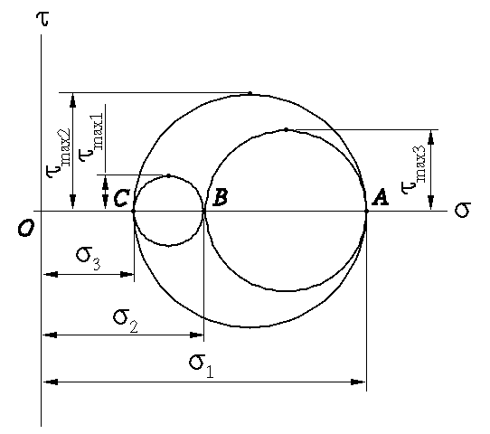
What if the rotations are about the axes rather than principal axes? It can be shown that any other transformation of axes would lead to stresses represented in Fig. 4 by a point located within the area which is bounded by the bigest circle with the other two circles removed!
Therefore, one can obtain the maxium/minimum normal and shear stresses from Mohr's circles for 3-D stress as shown in Fig. 4!
Note the notations above (which may be different from other references), one obtains that
Note that in Fig. 4, tmax1 , tmax2 , and tmax3 are the maximum shear stresses obtained while the rotation is about n1, n2, and n3 , respectively.
INPUT PARAMETERS :
1. For 2D Mohr circle, sigma x, sigma y and tau x i.e, Tensile stress, Compression stress (magnitude) shear stress are inputs for the 2D tensor.
2. For 3D Mohr circle, a 3 by 3 symmetric stress sensor are inputs.
PYTHON CODE :
1. For 2D Mohr circle
"""
Mohr circle in 2D.
"""
import numpy as np
import matplotlib.pyplot as plt
from matplotlib import rcParams
rcParams['font.family'] = 'serif'
rcParams['font.size'] = 16


def mohr(S):
    """Plot Mohr circle for a 2D tensor"""
    S11 = S[0][0]
    S12 = S[0][1]
    S22 = S[1][1]
    center = [(S11 + S22)/2.0, 0.0]
    radius = np.sqrt((S11 - S22)**2/4.0 + S12**2)
    Smin = center[0] - radius
    Smax = center[0] + radius

    print("Minimum Normal Stress: %g" % Smin)
    print("Maximum Normal Stress: %g" % Smax)
    print("Average Normal Stress: %g" % center[0])
    print("Minimum Shear Stress: %g" % -radius)
    print("Maximum Shear Stress: %g" % radius)

    circ = plt.Circle((center[0],0), radius, facecolor='#cce885', lw=3,
    edgecolor='#5c8037')
    plt.axis('image')
    ax = plt.gca()
    ax.add_artist(circ)
    ax.set_xlim(Smin - .1*radius, Smax + .1*radius)
    ax.set_ylim(-1.1*radius, 1.1*radius)
    plt.plot([S22, S11], [S12, -S12], 'ko')
    plt.plot([S22, S11], [S12, -S12], 'k')
    plt.plot(center[0], center[1], 'o', mfc='w')
    plt.text(S22 + 0.1*radius, S12, 'A')
    plt.text(S11 + 0.1*radius, -S12, 'B')
    plt.xlabel(r"$\sigma$", size=18)
    plt.ylabel(r"$\tau$", size=18)
    plt.show()
    return None

ts = float(input('Enter tensile stress(magnitude) in kPa at given state:'))
ss = float(input('Enter shear stress(magnitude) in kPa at given state:'))
cs = float(input('Enter compression stress(magnitude) in kPa at given state:'))
cs = -cs

S = np.array([[ts, ss],[ss, cs]])
mohr(S)
2. For 3D Mohr circle
"""
Mohr circle in 3D.
"""

import numpy as np
import matplotlib.pyplot as plt
from scipy.linalg import eigvalsh
from matplotlib import rcParams

rcParams['font.family'] = 'serif'
rcParams['font.size'] = 16


def plot_mohr3d(S):
    """Plot 3D Mohr circles."""

    S3, S2, S1 = eigvalsh(S)

    R_maj = 0.5*(S1 - S3)
    cent_maj = 0.5*(S1+S3)

    R_min = 0.5*(S2 - S3)
    cent_min = 0.5*(S2 + S3)

    R_mid = 0.5*(S1 - S2)
    cent_mid = 0.5*(S1 + S2)

    circ1 = plt.Circle((cent_maj,0), R_maj, facecolor='#cce885', lw=3,
                       edgecolor='#5c8037')
    circ2 = plt.Circle((cent_min,0), R_min, facecolor='w', lw=3,
                       edgecolor='#15a1bd')
    circ3 = plt.Circle((cent_mid,0), R_mid, facecolor='w', lw=3,
                       edgecolor='#e4612d')

    print("Minimum Normal Stress: ",float(cent_maj) - float(R_maj))
    print("Maximum Normal Stress: ", float(cent_maj) + float(R_maj))
    print("Average Normal Stress: ", float(cent_maj))
    print("Minimum Shear Stress: ", float(-R_maj))
    print("Maximum Shear Stress: ", float(R_maj))

    plt.axis('image')
    ax = plt.gca()
    ax.add_artist(circ1)
    ax.add_artist(circ2)
    ax.add_artist(circ3)
    ax.set_xlim(S3 - .1*R_maj, S1 + .1*R_maj)
    ax.set_ylim(-1.1*R_maj, 1.1*R_maj)
    plt.xlabel(r"$\sigma$", size=18)
    plt.ylabel(r"$\tau$", size=18)
    #plt.savefig('Mohr_circle_3D.svg')
    plt.show()

ts = float(input('Enter tensile stress(magnitude) in kPa at given state:'))
ss = float(input('Enter shear stress(magnitude) in kPa at given state:'))
cs = float(input('Enter compression stress(magnitude) in kPa at given state:'))


S = np.array([
    [ts,ss,0],
    [ss,cs,0],
    [0,0,0]])

plt.figure()
plot_mohr3d(S)
RESULTS :
1. For 2D Mohr Circle
For sigma x = 100 kPa; For sigma y = -60 kPa; For tau xy = 48 kPa;
Validation of results :
1. For 3D Mohr Circle
For sigma xx = 6 kPa; For tau xy= -3 kPa; For tau xz = 0 kPa;
For tau yx= -3 kPa; For sigma yy = 3.5 kPa; For tau yz = 0 kPa;
For tau zx= 0 kPa; For tau zy= 0 kPa;For sigma zz = 0 kPa;
Validation of results :
CONCLUSION :
Mohr circle has a great significance in the study of solid mechanics. Mohr’s circle has been used as a graphical method for performing coordinate transformations for stress, but the technique applies equally well to any 2x2 tensor matrix. Mohr’s circle also provides rapid graphical estimations for eigenvalues and eigenvectors, which is extremely useful for verifying analytical results. Mohr’s circle is not just for stress tensors, but it is typically taught in only that context in introductory materials mechanics courses. For stress tensors, Mohr’s circle can be used to visualize and to determine graphically the normal and shear stresses acting on a plane of any given orientation. For symmetric tensors, Mohr’s circle can be generalized to 3x3 matrices for a graphical depiction of the set of all possible normal and shear components. The traditional definition of Mohr’s circle for symmetric matrices is presented with numerous examples for performing coordinate transformations, finding the plane(s) of maximum shear, and identifying eigenvalues and eigenvectors. An important but little-known enhancement to Mohr’s circle (called the Pole Point) is shown to rectify counter-intuitive factors of 2 when converting angles in physical space to angles in the Mohr diagram. The extension of Mohr’s circle to 3x3 matrices is presented with application to the Mohr-Coulomb theory of material failure. The basic construction of Mohr’s circle is shown to apply with only minor modification to nonsymmetric matrices, in which case the circle no longer remains symmetric about the normal axis. Applications of nonsymmetric. Mohr’s circle include rapid eigenvalue/eigenvector determination and fast polar decompositions for deformation matrices. A numerical exploration is presented that suggests there is no simple extension of Mohr’s circle to 3x3 nonsymmetric matrices. Hence, this project helps to determine the principal stresses by using Mohr Theory with limited inputs.