AIM: To Run a pipe flow simulation with an inlet Reynolds number of 100,1000 and 10,000.

Objectives of the challenge:

• To run an internal pipe flow simulation with an inlet Reynolds number of 100, 1000 and 10,000 .
• For each of these cases we need to –
1. Place line probes at 95%, 90% and 85% of the pipe length.
2. Compare the normalized velocity profile at each of these locations.
3. Normalize the velocity profile by the inlet velocity.

Introduction:

The definition of a flow is an act of moving or running smoothly, a movement of water or the continuous moving of ideas, stories, etc. The substances which have the tendency to flow is also called as fluid.

Fluid Flow Simulation:

Computational Fluid Dynamics (CFD) is the branch of CAE that simulates fluid motion and heat transfer using numerical approaches. Carrying out fluid flow simulation in a virtual environment is a better suited approach. This allows the engineers to model the fluid’s behavior at every stage in the process and accurately predict how it will react in an actual casting environment. In doing so, it greatly reduces the time it takes to create a working design, which can then be manufactured in the real world. Because of the work that has been done in the virtual world, the chances of this unit performing as excepted are greatly increased and the overall cost of development is substantially reduced.

Types of Fluid Flow:

There are Six different types of fluid flow:

• Steady and Unsteady
• Uniform and Non-Uniform
• Laminar and Turbulent
• Compressible and In-compressible
• Rotational and Ir-rotational and
• One, Two, and Three -dimensional Fluid Flow

Our main course of interest:

• Laminar and Turbulent fluid flow: - This laminar fluid flow is defined as the type of flow in which the fluid particles move along well-defined paths or streamline and all the streamlines are straight and parallel.

Thus, the particles move in laminas or layers gliding smoothly over the adjacent layer. This type of fluid is also called as streamline flow or viscous flow.

This Turbulent fluid flow is defined as the type of flow in which the fluid particles move in a zig-zag way, the eddies formation takes place which is responsible for high energy loss.

Reynolds Numbers

Fluid flow in a pipe encounters frictional resistance due to the internal roughness (e) of the pipe wall, which can create local eddy currents within the fluid. Calculation of the Reynolds Number helps to determine if the flow in the pipe is Laminar Flow or Turbulent Flow.

"Re = " ρuD/μ = uD/ν`

• ρ is the density of the fluid (SI units: kg/m³)
• u is the flow speed (m/s)
• D is the diameter of the tube (m)
• μ is the dynamic viscosity of the fluid (Pa·s or N·s/m² or kg/(m·s))
• ν is the kinematic viscosity of the fluid (m²/s) .

The Kind of flow is based on the value of Re ,

> If Re < 2000, the flow is called Laminar flow

> If Re > 4000, the flow is called Turbulent flow

> If 2000 < Re < 4000, the flow is called transition.

Procedure:

1. A rod of 0.05m diameter and 1m in length was created. Using the shell feature, we have generated the required thickness of 0.001m.

   

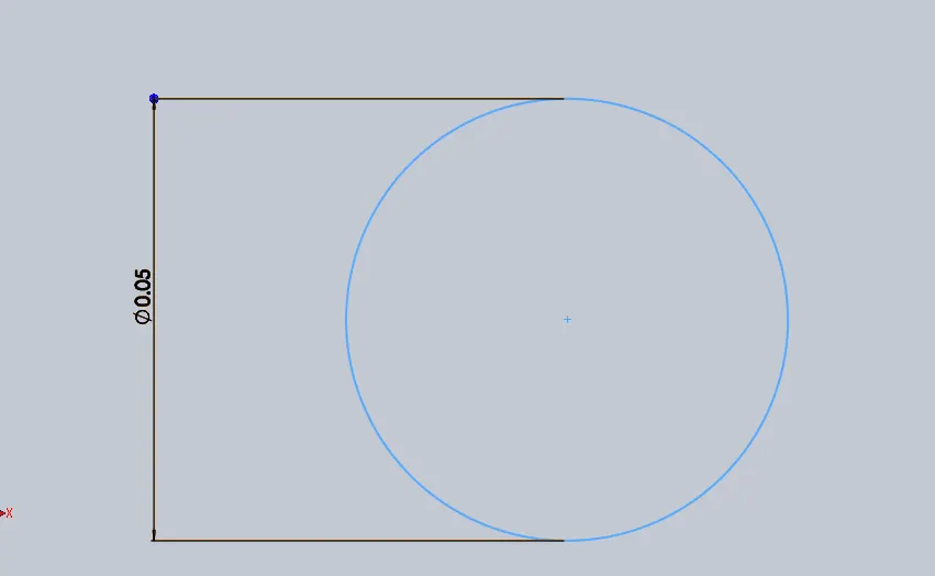
2. Line probes were drawn at the top plane for 85, 90, and 95% of length i.e 0.85m, 0.90m, and 0.95m respectively.
3. Lids were provided at both ends to make sure that the pipe is closed.
4. Choosing wizard option, clicking internal flow, initial temp is 293.2K AND 1010325Pa with air as a working fluid
5. Using global mesh, it is manually defined as 20 in the X direction, 20 in the Y direction, and 100 in the Z direction.

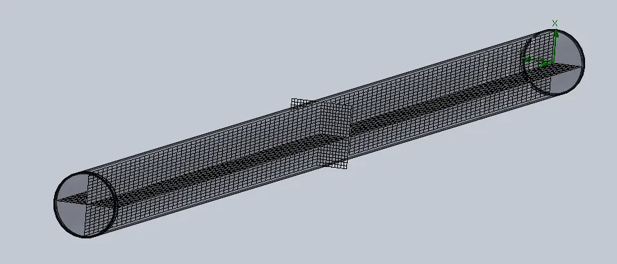
6. Providing inlet velocity and static pressure at outlet along with defining walls as a real wall, all this helps us to define the boundary conditions.

Inlet velocity was determined using the above formula and values used are mentioned below in the table.

Flow diameter of the pipe = 0.03- 2*(0.001) = 0.028m (Characteristic Length)

μ= 18.03 * 10^-6 Pa-s (Dynamic Viscosity)

Reynold's No.	Velocity
100	0.00185 m/s
1000	0.0185 m/s
10000	0.185 m/s

7. After completing the simulation, the XY plots were plotted for various probes to compare the velocity profile and get a better understanding

OBSERVATIONS, RESULTS AND CONCLUSION:

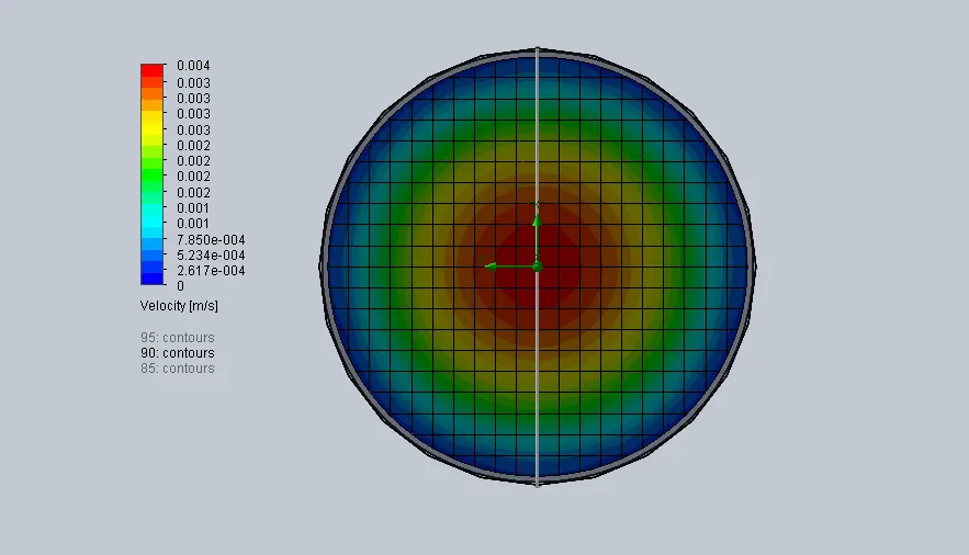
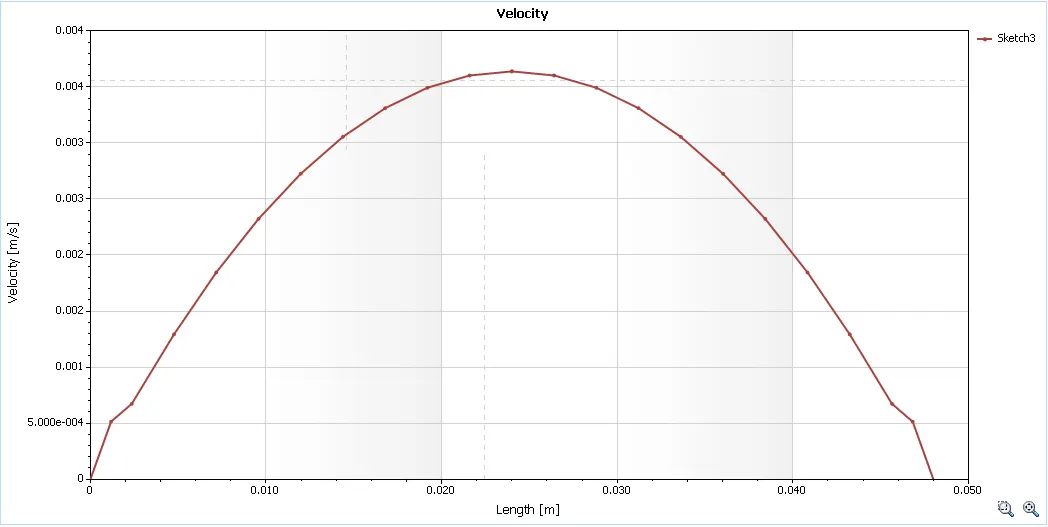
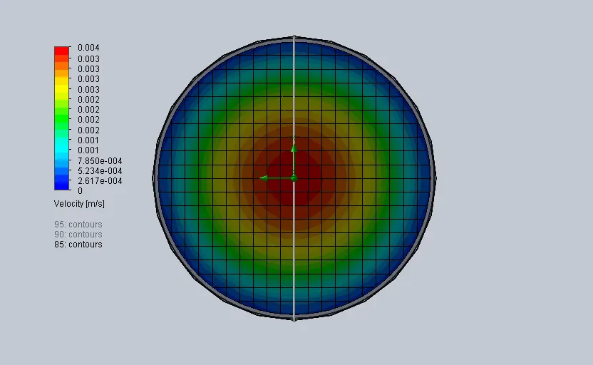
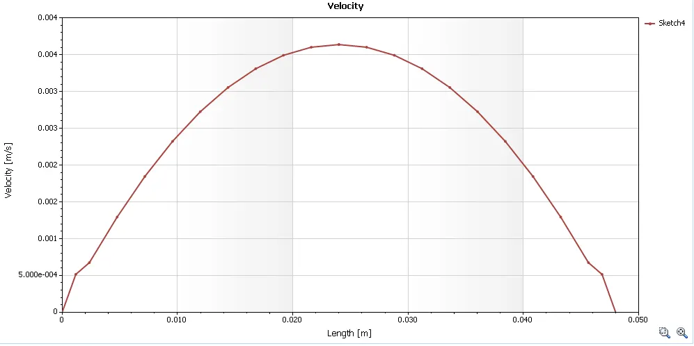
Study-1: Pipe flow simulation with inlet Reynolds number (Re) = 100 & flow speed (u) = 0.00185 m/s

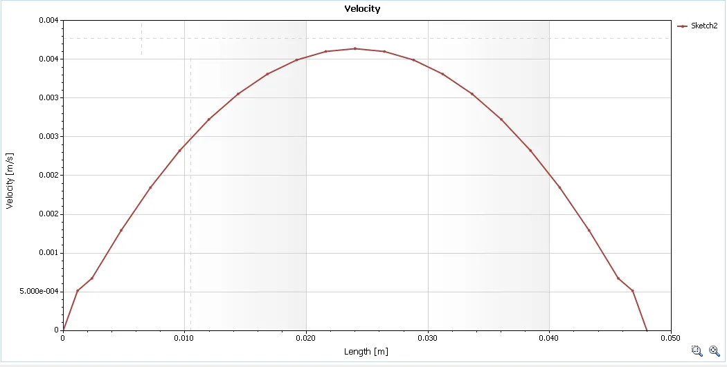
• At line probe 95

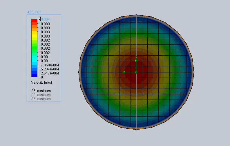
Velocity plot:

• At line probe 90

Velocity plot:

• At line probe 85

Velocity plot:

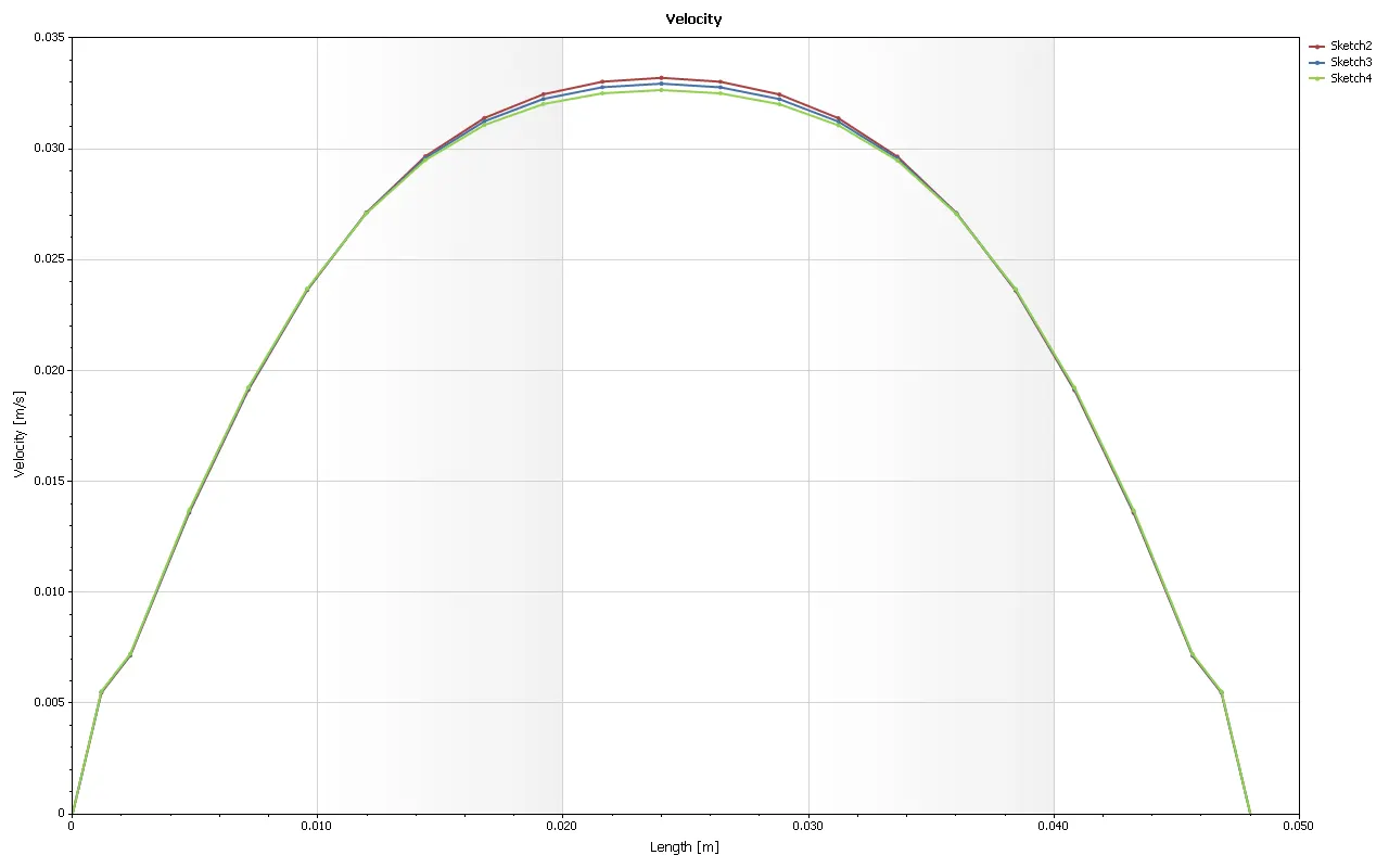
Velocity comparison plot:

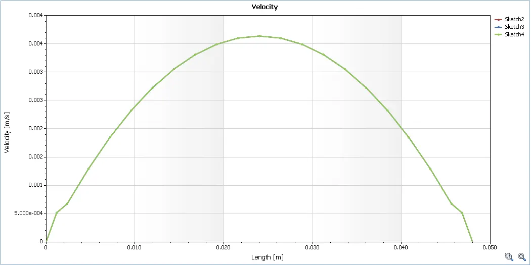
• Sketch 2 represent velocity at probe 95
• Sketch 3 represent velocity at probe 90
• Sketch 4 represent velocity at probe 85

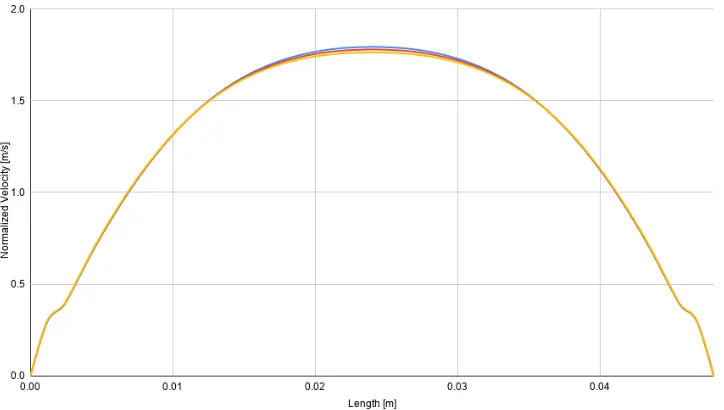
Normalized velocity plot:

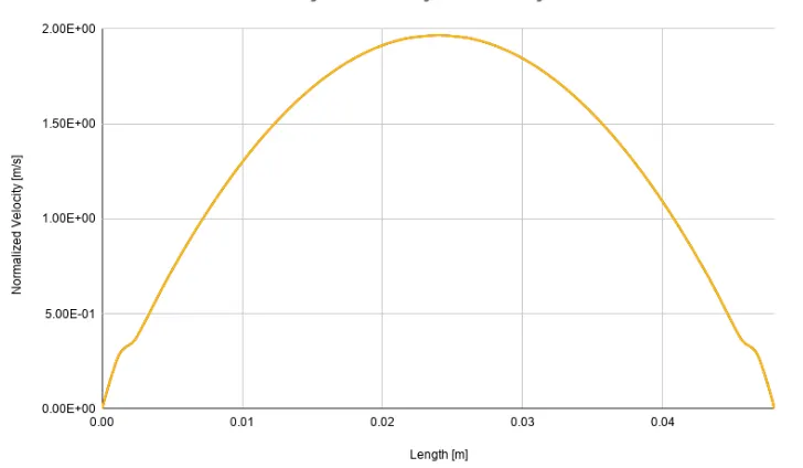
Observation are that the cut plot is similar for the 3 different probe lengths, as this case comes under laminar flow. The velocity profile is parabolic in nature and can be seen in overall velocity distribution. Velocity is maximum at the center as the least shear resistance is offered there and minimum at the boundary.

Study-2: Pipe flow simulation with inlet Reynolds number (Re) = 1000 & flow speed (u) = 0.0185 m/s

AT Line Probe at 95% -

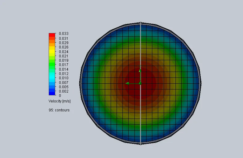
Velocity plot:

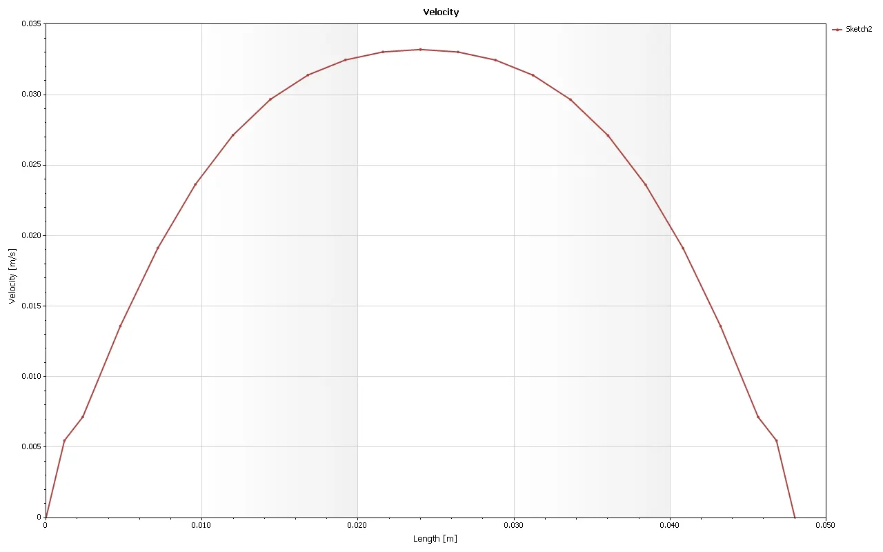
AT Line Probe at 90% -

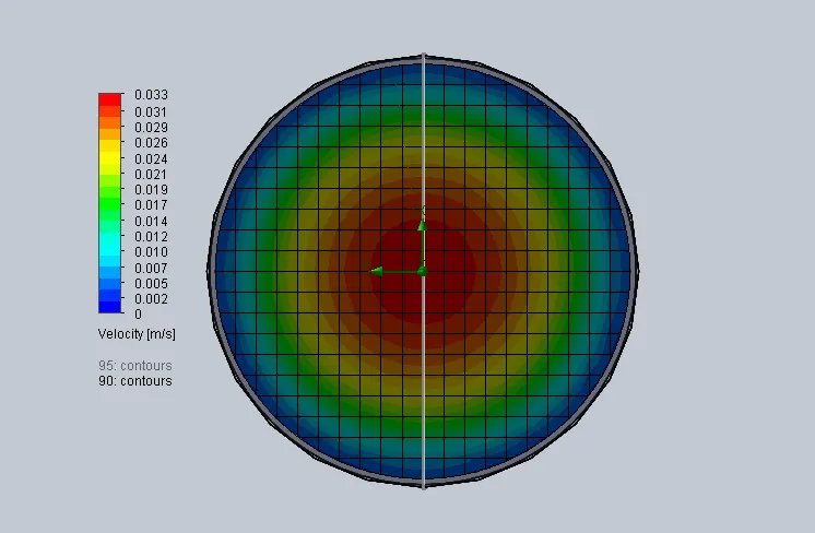
Velocity plot:

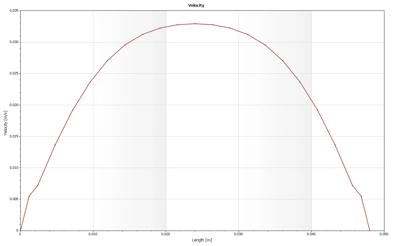
AT Line Probe at 85% -

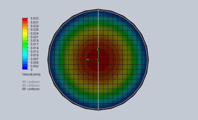
Velocity plot:

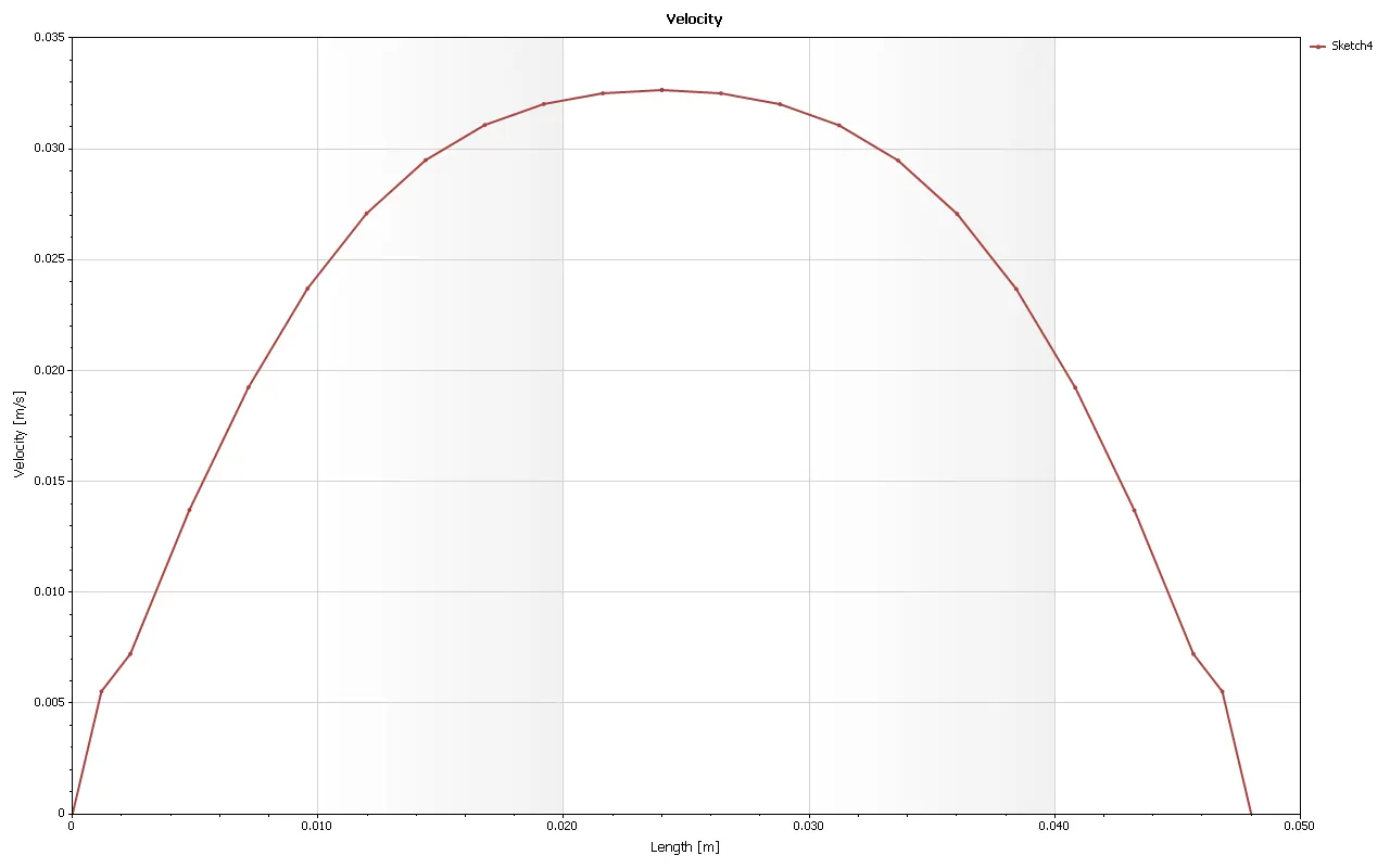
Velocity comparison plot:

• Sketch 2 represent velocity at probe 95
• Sketch 3 represent velocity at probe 90
• Sketch 4 represent velocity at probe 85

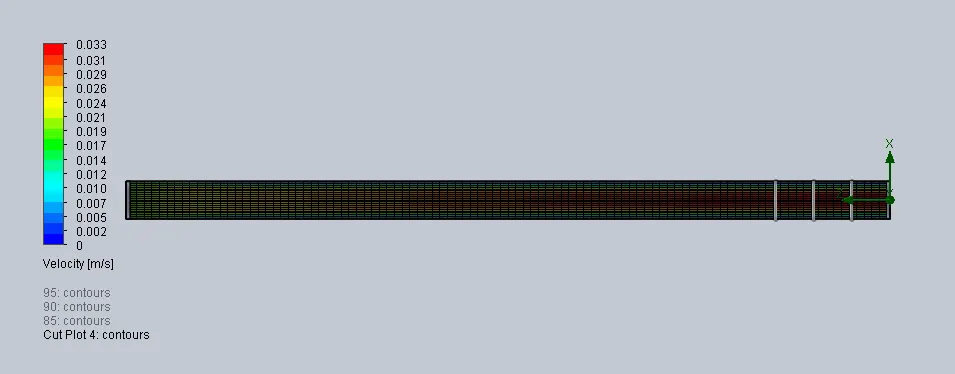
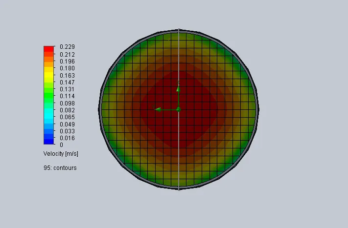
We can say that as reynolds number increases, the turbulance of the flow also increases and the working fluid is mixed more and more and thus the effect of viscosity and the effect of friction near the walls gets lesser and lesser. Thus we can see less of the blue color in the third image and more of blue color in the first image indicating low velocity.

Study-3: Pipe flow simulation with inlet Reynolds number (Re) = 10,000 & flow speed (u) = 0.185 m/s

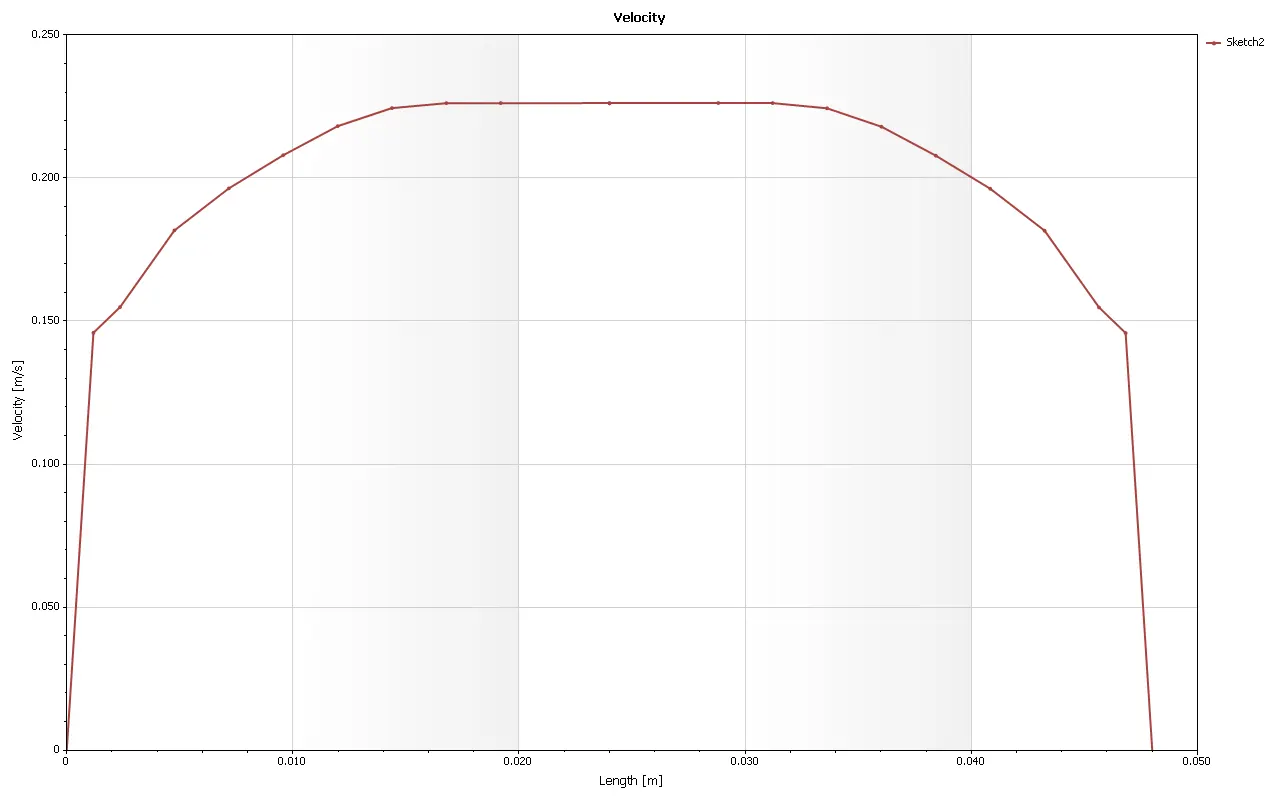
At line Probe at 95% -

Velocity:

At line Probe at 90% -

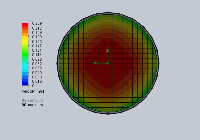
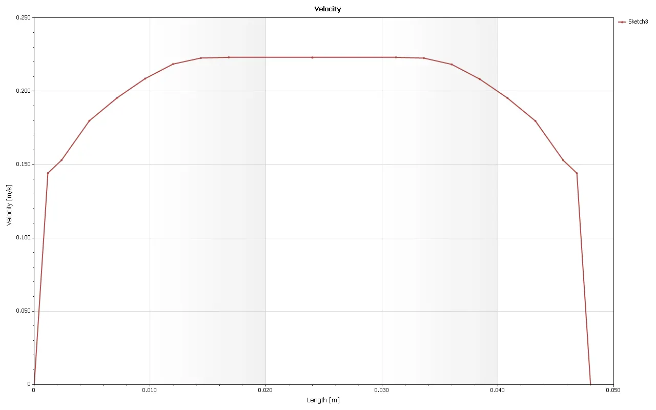
Velocity plot:

At line Probe at 85% -

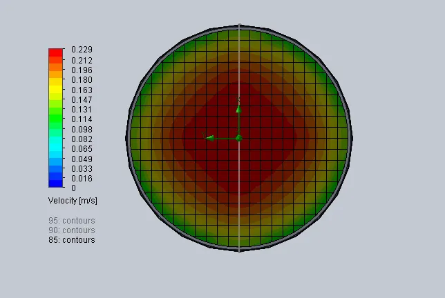
Velocity plot:

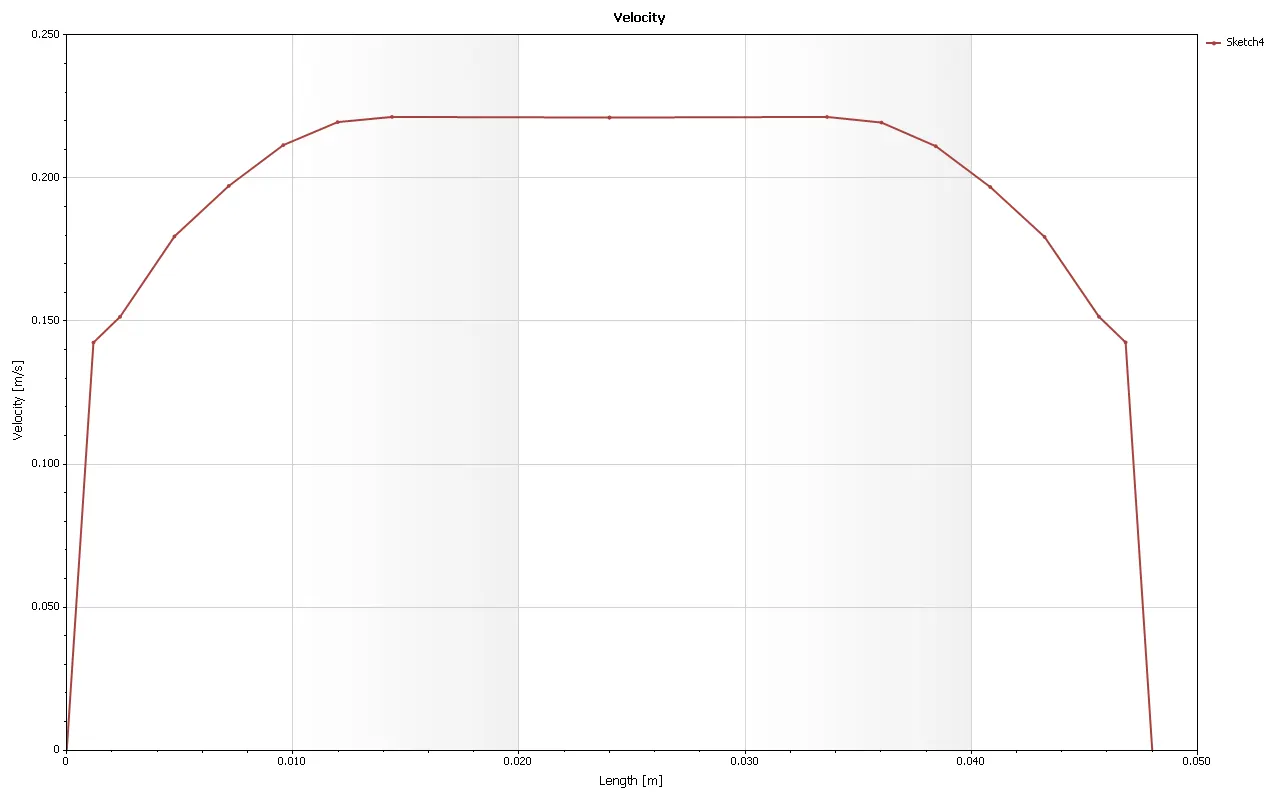
Velocity comparison:

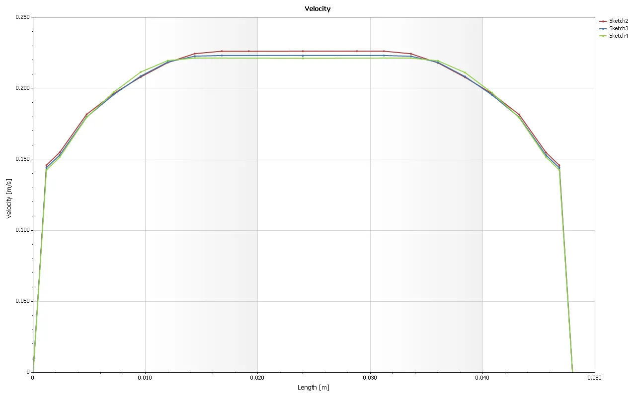
• Sketch 2 represent velocity at probe 95
• Sketch 3 represent velocity at probe 90
• Sketch 4 represent velocity at probe 85

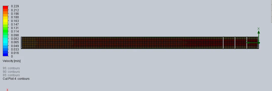
We can see that the velocity profiles at all the line probes are overlapping each other with a higher accuracy. But velocity in the middle section or at the centre of the pipe is varying. That velocity is directly proportional to the distance from the inlet of the pipe. Thus we can say that at a middle ground laminar flow, the velocity is not affected much starting from the pipe wall upto a distance of approximately `D/4`. The red region is affected and as mentioned above, the velocity changes (increases). The red region approximately covers a distance of `D/2`. Notable thing is that velocity at walls is "equal to" Zero.

Conclusion:

Flow varies from 0 at the initial surface to the maximum at the center. This is because we know that it follows a parabolic profile according to which least offered resistance is at the center and velocity is maximum there.Also with increase in Reynolds number, velocity gets more uniform.

Moreover, one more thing to notice is that velocity near the boundary is tending to zero, the main reason is the formation of the boundary layer near the surface.