Gate Valve Parametric Study

Parametric analysis on gate valve

Aim:-

To perform a parametric analysis on the gate valve simulation by setting the opening from 10% to 80%. Obtaining the result for mass flow at the outlet for each opening with flow coefficient and flow factor.

Introduction:-

Valves control the fluid flow and pressure in a system or a process. The selection of their types, design and material plays a vital role in the performance and reliability of any system. A number of researchers have experimented and analyzed valves for all its parts, fluid types, operating parameters, discharge coefficient, stiction and eroding characteristics and have improved the valve technology. Now, with the emergence of robust computational fluid dynamics (CFD) tools and powerful computers, the analysis of valve performance, and thus the job of designing valves to suit a particular application can be done much faster. Apart from this, CFD analysis can reveal the complex flow structure and the sonic characteristics around the valve, which the experiments hardly provide. Even otherwise, experimentation needs to be supplemented with CFD analysis because of the complex geometry as well as complexities like turbulence during the sonic flow through a valve. The experimental results were validated by CFD analysis or vice versa. In the present study, CFD analysis of a specific globe valve design has been carried out to understand its performance and reliability during the high pressure flow of gaseous oxygen.

A gate valve is a type of flow control device that controls the flow of gas, oil or water. Gate valve analysis in the past was performed using experiment methods, which required a number of equipment, a lot of time, fund and so on. It is not a good way to investigate the flow characteristic of an actual prototype of any

valve in a laboratory. Nowadays, due to the fast progress of the computer visualization and numerical techniques, it becomes possible to do it by using simulation technique. Another method wherein valve performance factors can be obtained is by using Computational Fluid Dynamics (CFD) software to simulate the physics of fluid flow in a piping system around a valve. However, only studying the fluid characteristics is not enough for gate valve because, the pressure produced by the fluid is too high, which has great effect on the stress distribution in valve. Fluid Structure Interaction (FSI) occurs when the flow of fluid influences the properties of a structure or vice versa. It is a great challenge to deal with such problems due to its complexity in defining the geometries, nature of interaction between a fluid and solid, multi-physics facts and requirements of computational resources. It is tedious, time consuming and challenging work for a designer to measure the accurate stress distribution of any mechanical component which results in some deficiencies in the design of that particular component. To overcome these deficiencies, computer aided software like ANSYS, CATIA, SOLIDWORKS are used. According to the Research, analysis and optimization can be done by using analysis software for greater accuracy and also to minimize the time of designer.

Theory:-

Gate valves are machine elements which are commonly used to control the flow of fluids as gate valve provides a positive sealing at high pressure of liquids and gases. Gate valves are used when a straight-line flow of fluid and minimum restriction is desired. Gate valves are so named because the part that either stops or allows flow of fluid through the valve acts somewhat like the opening or closing of a gate and is called, appropriately, the gate. The objective of this paper is to focus the design and analysis of critical components of Gate Valve. The critical components in the Gate Valve studied by many of the researchers are Body, Gate Stem and slab gate. The main purpose of design and analysis of any valve is to determine stresses and strains developed in the valve body, which is mostly done by using computer aided software tools.

There are different kinds of valves available and each one is used for a specific purpose . Gate valves are generally used in systems where low flow resistance for a fully open valve and no throttling are desired. Globe valves are used in systems where good throttling characteristics and low seat leakage are desired with relatively high head loss allowable in an open valve. Ball valves allow quick, quarter turn on-off operation and have poor throttling characteristics. Plug valves are used for changing flow direction between different ports via a single valve. Diaphragm valves and pinch valves are used in systems wherein the system is required to

be completely isolated from the fluid. Butterfly valves provide significant advantages over other valves in weight, space, and cost for large valve applications. Check valves are used in applications where open flow in one direction and prevention of flow in the reverse direction are desirable. A combination of characteristics of lift check valve and a globe valve gives a stop check valve. Safety relief valves are used to provide automatic protection for over-pressurization in a system. Researchers have extensively experimented with all the above

categories of the valves in order to identify the valves for specific applications. The computational

analyses have not been performed that extensively as the experimental study. The application of valves in high pressure and high flow rate gaseous streams calls for thorough research and analysis. The methodology adopted in these systems focus on the analyses, design and then experimental validation of the analysed results.

Valves, when used in high pressure systems, often get damaged by the frequent and severe movement of the metal pieces, back and forth, against each other over an extended period of time and by shock waves during the closing of the valves. Leakage is another problem in the valves used in high pressure systems. The repair or replacement requires demounting of the valve from an existing piping structure. The inconvenience and attendant damage to the surrounding piping structure poses major impediment to the valve replacement.

Another shortcoming in the valves employed in high pressure applications is the requirement of considerable pressure for actuating the valve. This is because the high seal pressure and related high friction forces are necessary to insure sealing. Further, the contaminants affect the seal life so severely that the life of the valves reduces to nearly half of its prescribed life time. In addition to all these, the geometry of the valve and the drop in velocity around the downstream region involves the risk of particle accumulation.

Globe valve is commonly used as the control valve for high pressure system due to lesser leakage and higher erosion resistance compared to other valves. Gate valves are good for low pressure systems and can perform efficiently without leakage only for low pressure systems. For high pressure systems, the vibration and shock waves due to the turbulence causes rapid erosion of the gate of the gate valve. This makes gate valve vulnerable to failure in high pressure gaseous systems.

Flow Coefficient () :-

The valve flow coefficient is an inherent parameter which measures the valve capacity. It depends on valve type, diameter of valve, opening rate of valve and operating fluids. Cv is defined as the floe in cubic meter per hour of water at a temperature 5-40°C with a pressure drop across the valve of 1 bar.

`Cv=Qsqrtfrac(SG) (DeltaP)`

Where

DP = pressure drop across the valve in psi.

SG = specific gravity of fluid.

Q = mass flow rate in US gallon per minute.

The metric equivalent of is , which is defined as the amount of water that will flow in with 1 bar pressure drop . converting between the two coefficient is based on this relationship.

`Cv=1.16Kv`

Pre-processing and meshing:-

A CAD geometry of Gate valve is imported from CAD package and uploaded to Spaceclaim as shown in Figure 1. In our present project we have to simulated the fluid flow inside the gate valve at different valve opening from 10% to 80%. To simulate a fluid inside the valve with different flow valve opening we have to parametrised the valve opening. This can be done by using a move option and then check it as a parameter. So every time when we change the value of valve height the actual geometry is change. In Spacecliam we have to extract the fluid volume by using a volume extract option. To update the geometry we have to right click on extract volume in tree and update volume body in context. The Figure 2 show the extracted fluid volume. Now from figure 3 to 10 shows the section view of extracted volume at different valve opening.

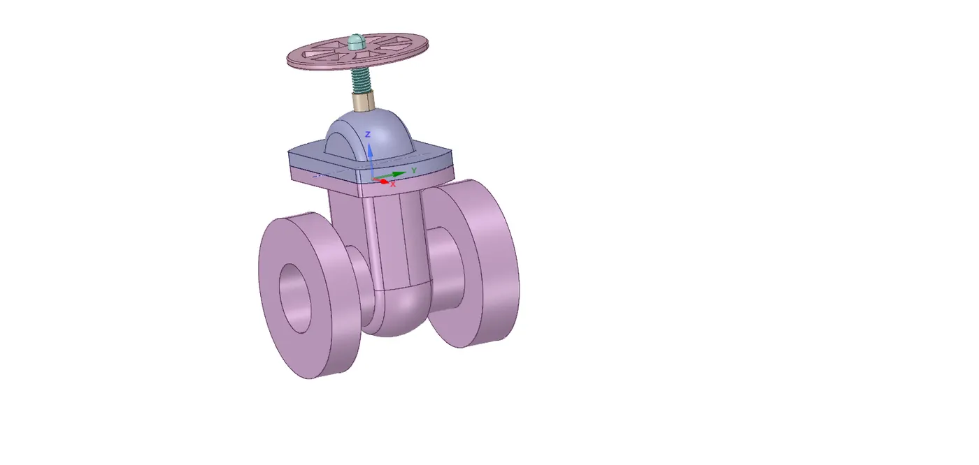
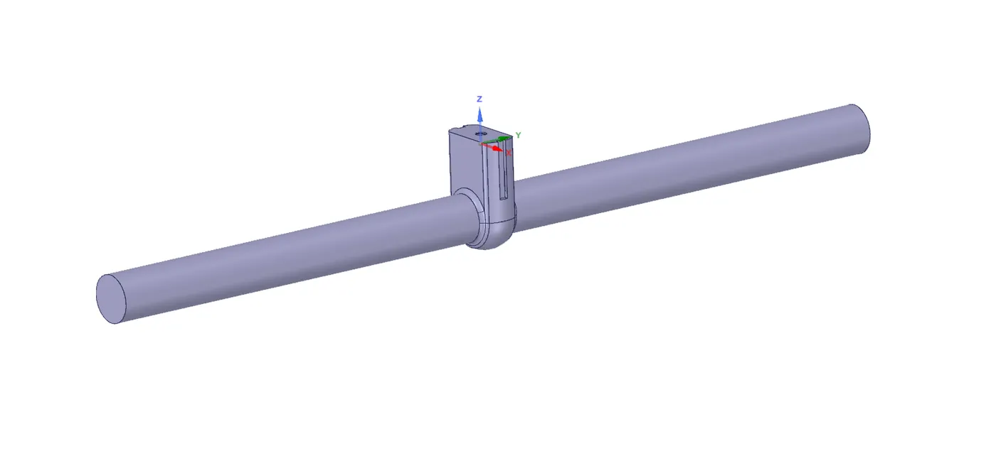
Figure 1, Gate valve geometry Figure 2, Extracted fluid volume

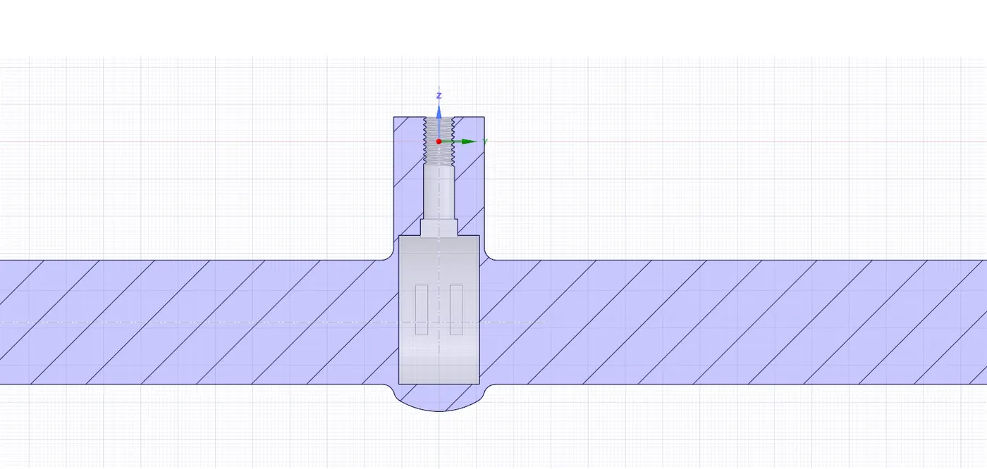
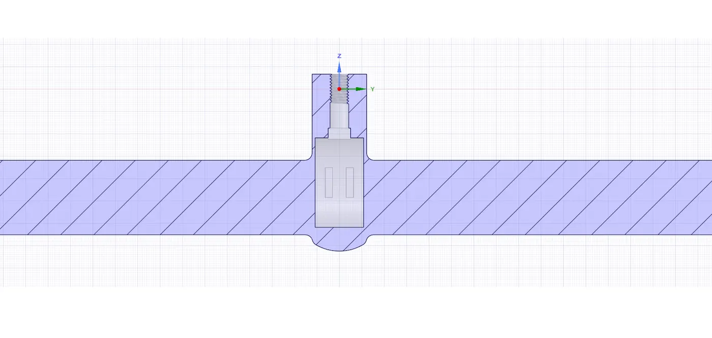
Figure 3, Valve opening of 10%. Figure 4, Valve opening of 20%.

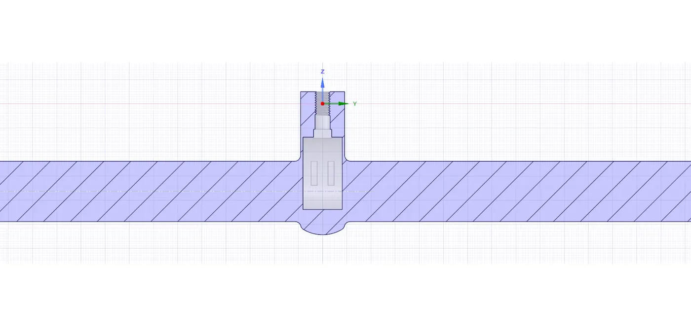
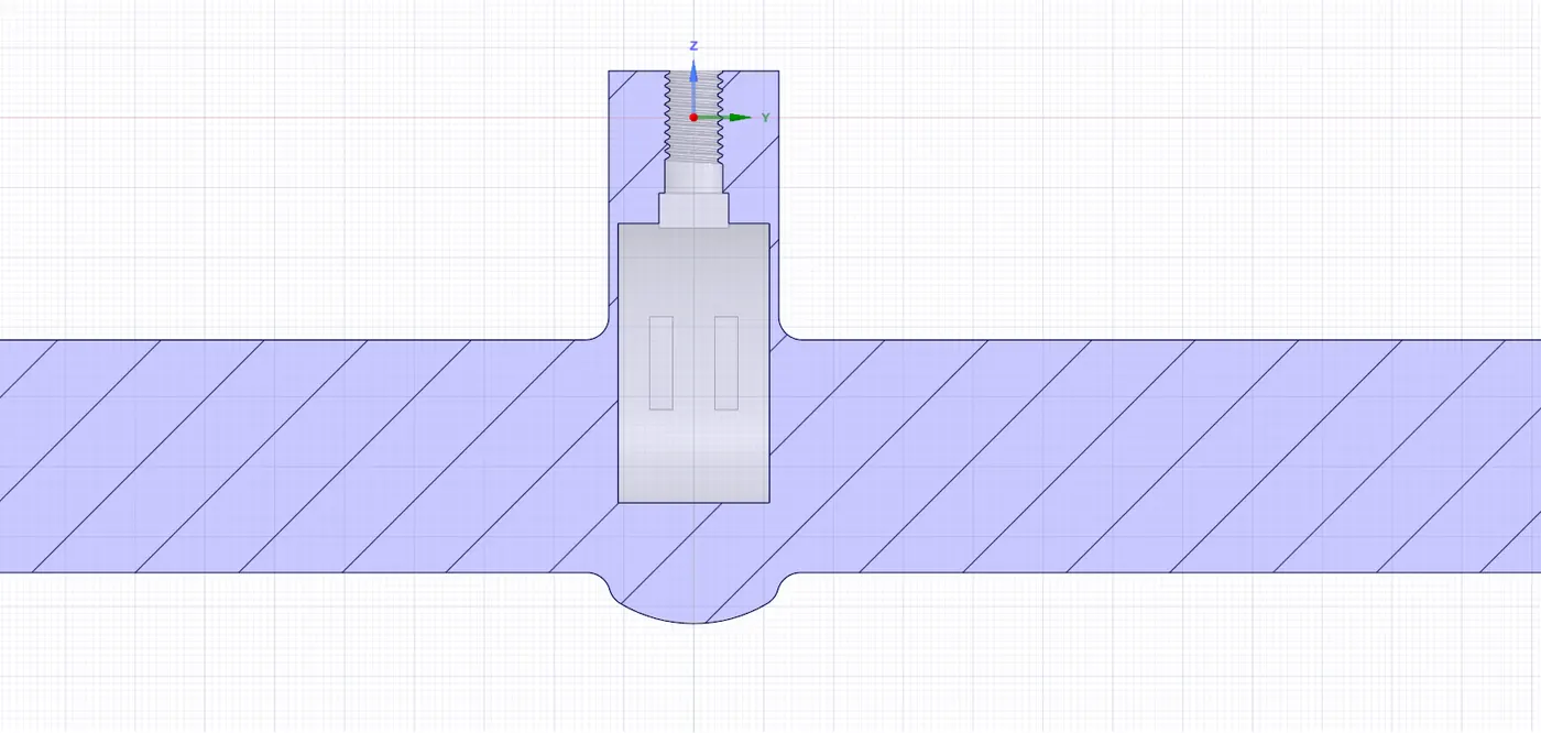
Figure 5, Valve opening of 30% Figure 6, Valve opening of 40%.

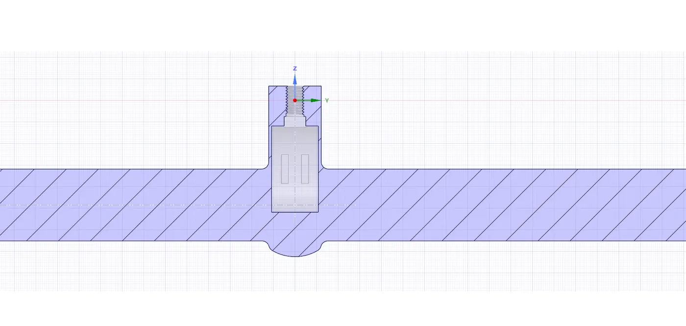
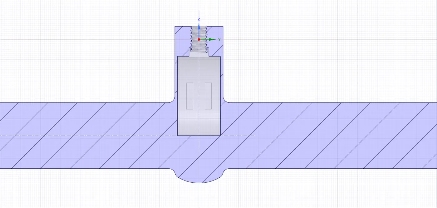
Figure 7, Valve opening of 50% Figure 8, Valve opening of 60%

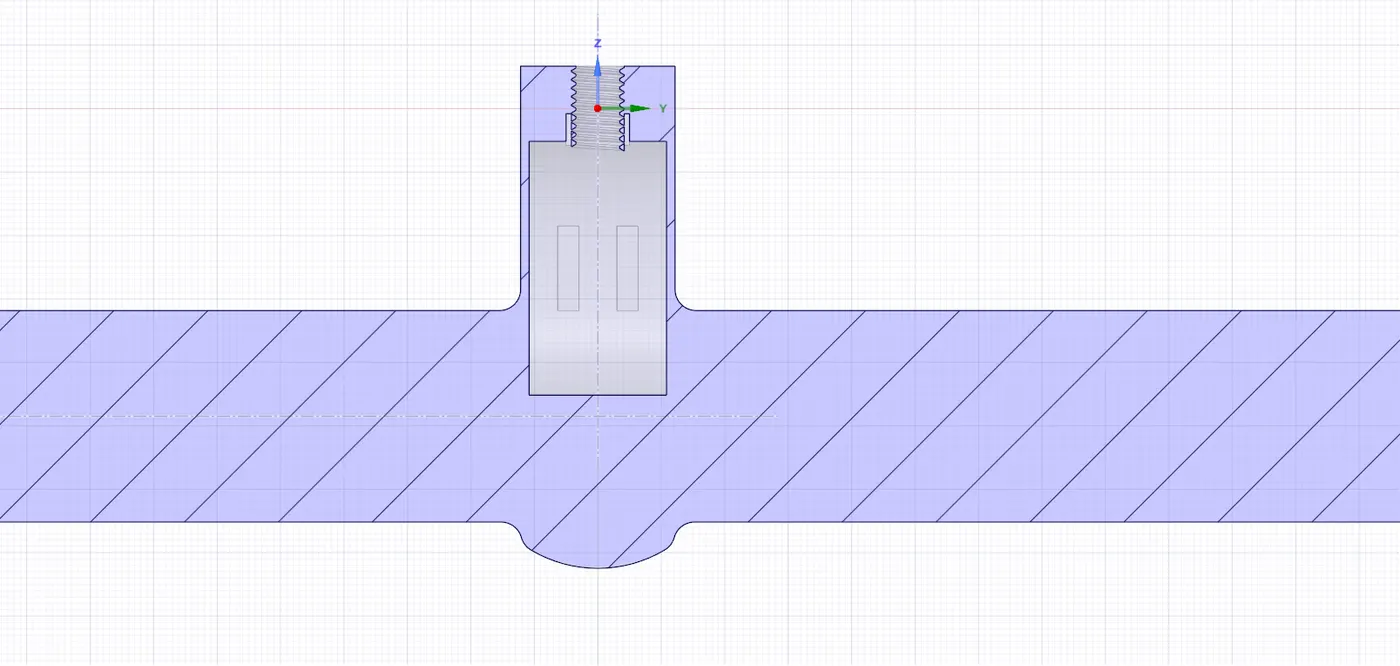
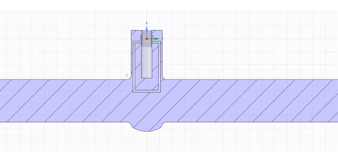
Figure 9, Valve opening of 70% Figure 10, Valve opening of 80%

After defining the geometry the file is uploaded for meshing. For meshing we choose trigonal mesh with element size of 14 mm. Figure 11 and 12 shows the meshed fluid volume and section view of fluid volume respectively. In our mesh the total number of element and nodes are 146969 and 31068. Inlet and outlet faces are defined using named selection tool as shown in Figure 13.

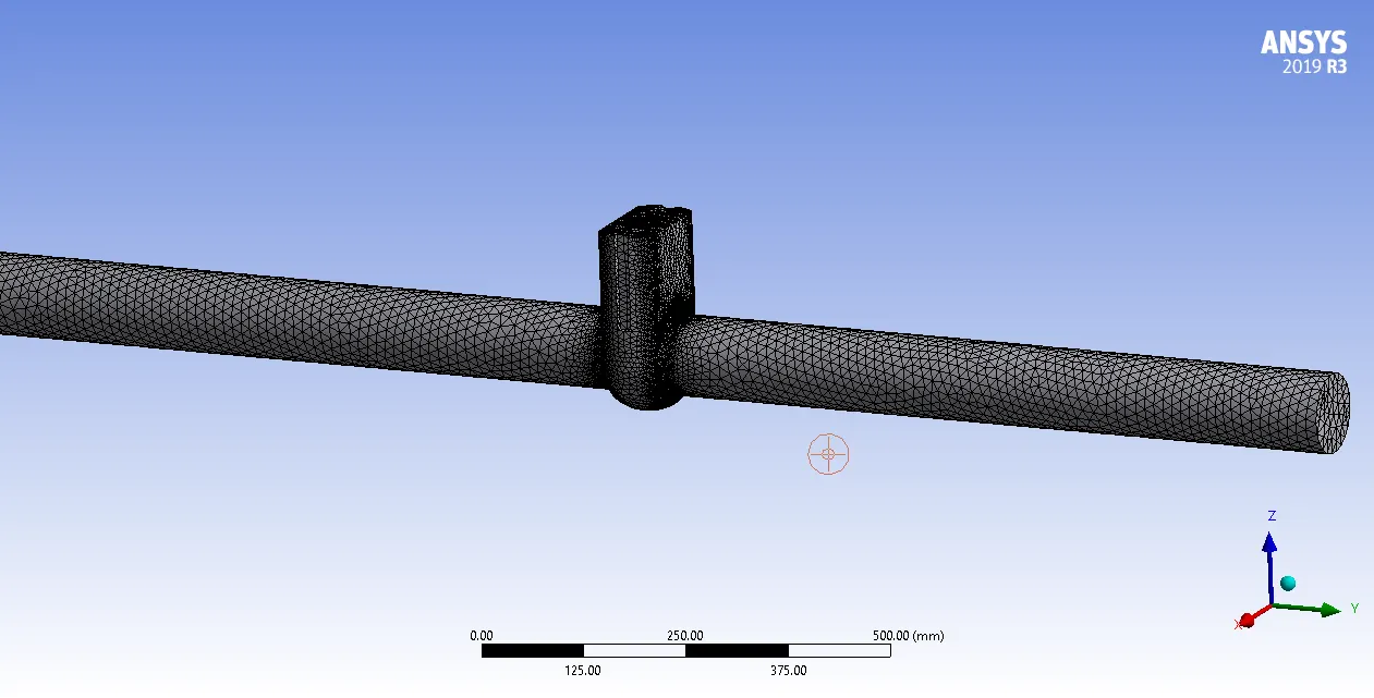
Figure 11, Meshed geometry.

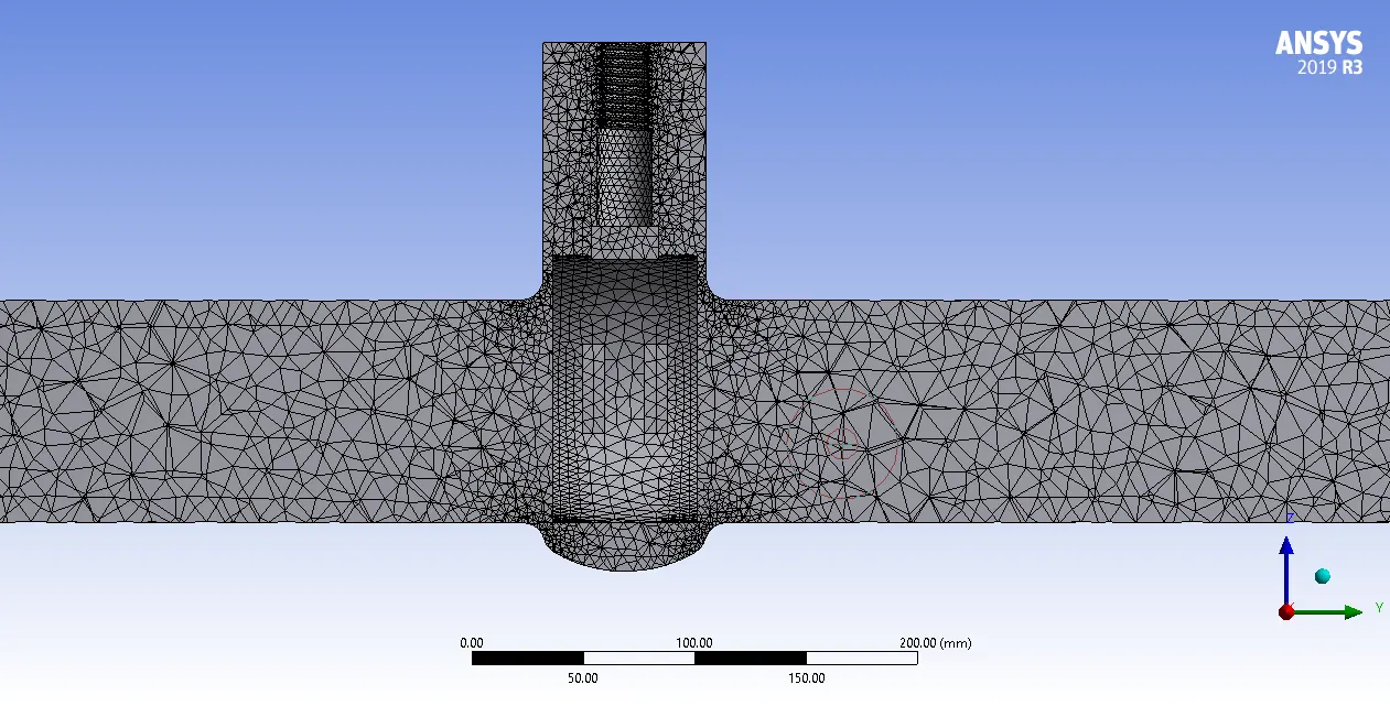
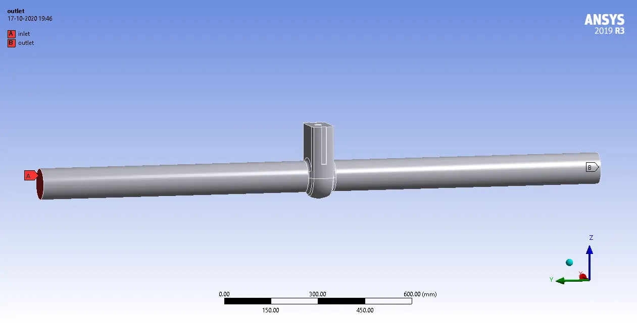
Figure 12, Section view of mesh. Figure 13, Geometry of named selection.

Solver setup:-

In fluent solver setup pressure based solver is used with steady state and gravity enables. In viscous

model Reliable K-e turbulent model is chosen with scalable wall function. Fluid material is chosen as water liquid from fluent database. In boundary condition inlet is pressure inlet with gauge pressure of 10 pascal. Outlet is selected as pressure outlet with gauge pressure of 0 because to make it as same as atmospheric pressure. Pressure velocity coupling scheme is chosen as Coupled with pressure and momentum of second order upwind. To track the convergence and accuracy of solution we have to add a flux report of mass flow rate at outlet. Then we have to create a two line one at upstream and one at downstream of valve at its mid plane as shown in Figure 14 . On this two line we collect a pressure data for this we have to create a surface report of facet average values on both line. To get a value of above mention report for different valve opening we have to check the create output parameter option. Initialized the solution by using standard initialization from inlet by this we can a inlet velocity. Then run the solution for 250 iteration. After completing the simulation we have to go to parameter tab and the change the value of input parameter from 10% to 80% and the update all design point. Then select on one design point and make it current. By this we can visualise the result from CFD post for selected case.

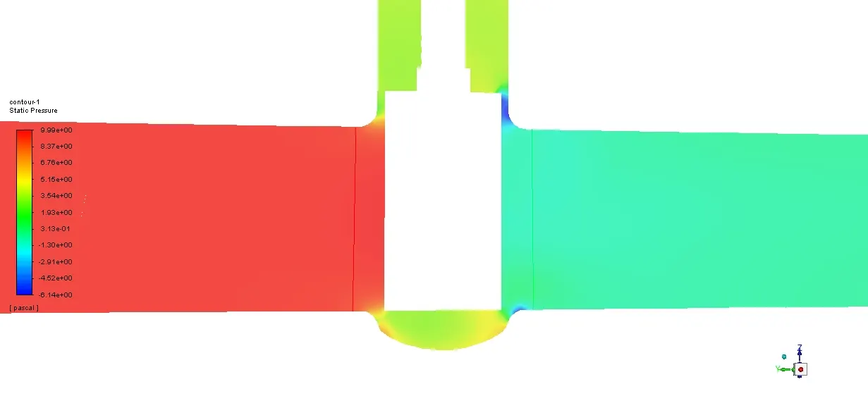
Figure 14, Line on Upstream and downstream of valve

Result:-

By making valve opening as input parameter we can calculated the data at different valve opening and make any design state as current and review fluid flow. As start from 10% to 80% of valve opening we can see from Figure 3 to 10. Residual plot of the 10% and 20% flow opening shows a continuous decrease in residual indicating a smooth convergence as shown in Figure 15 and 16. But from 30% to 80% of flow opening the residual are gaining a lot of fluctuation with high amplitude but as the iteration comes over 200 the frequency of amplitude is getting constant indicate that solution is reaching in steady state as shown in Figure 17 to 22. The mass flow at outlet is also plotted and the graph first reach at high value then it smoothly become constant and at last become a straight line shows the mass outlet is become constant as shown in Figure 23 to 30.

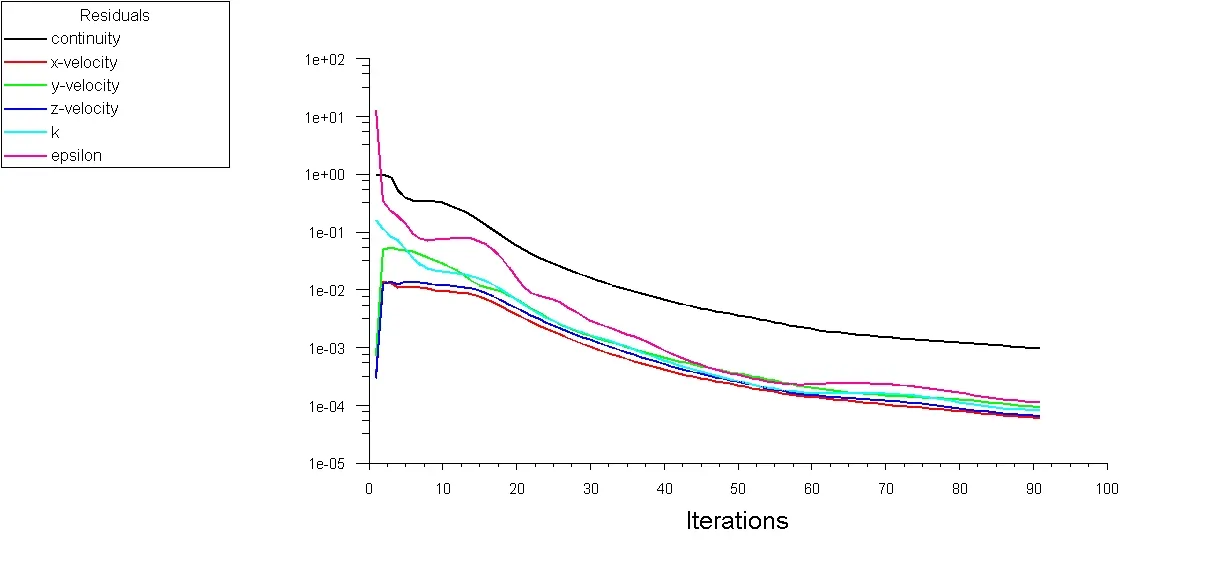
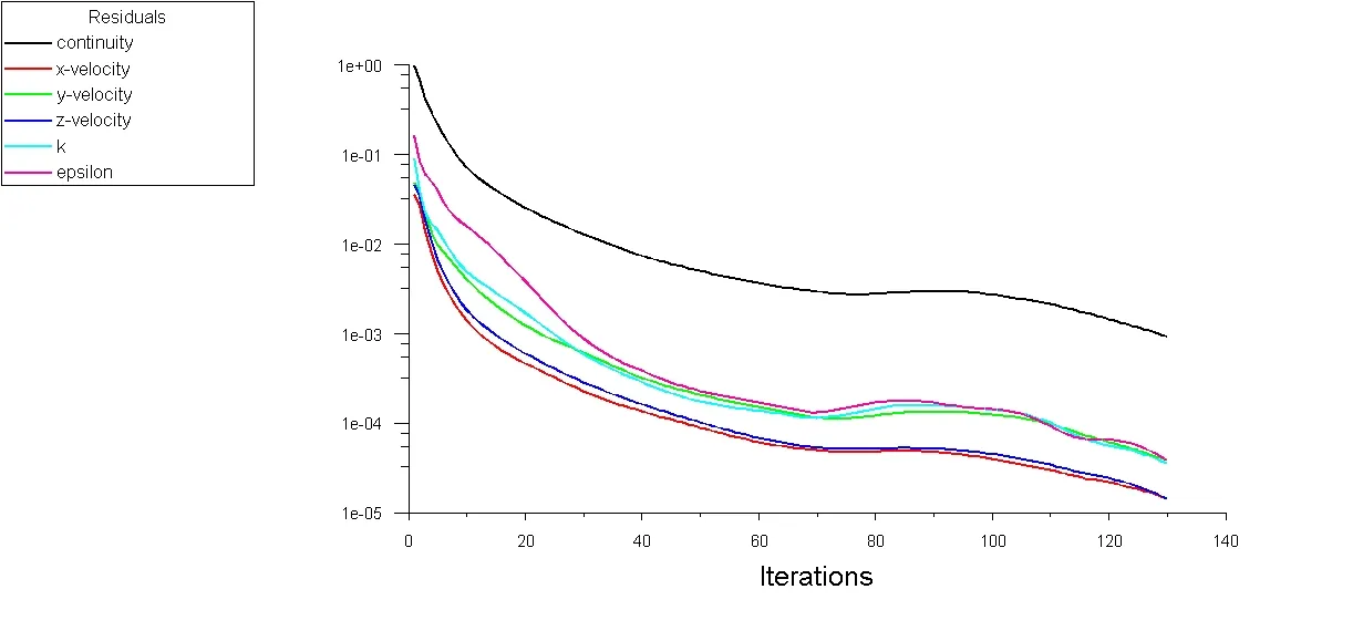
Figure 15, Convergence plot for 10% valve opening. Figure 16, Convergence plot for 20% valve opening.

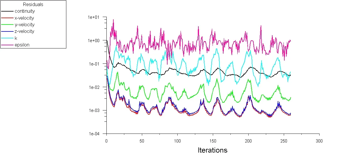
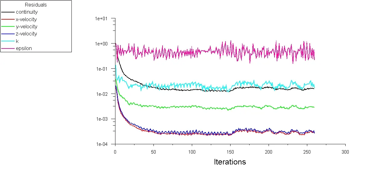
Figure 17, Convergence plot for 30% valve opening. Figure 18, Convergence plot for 40% valve opening.

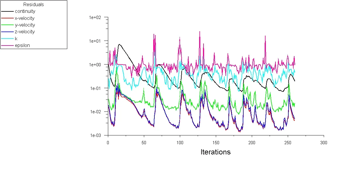
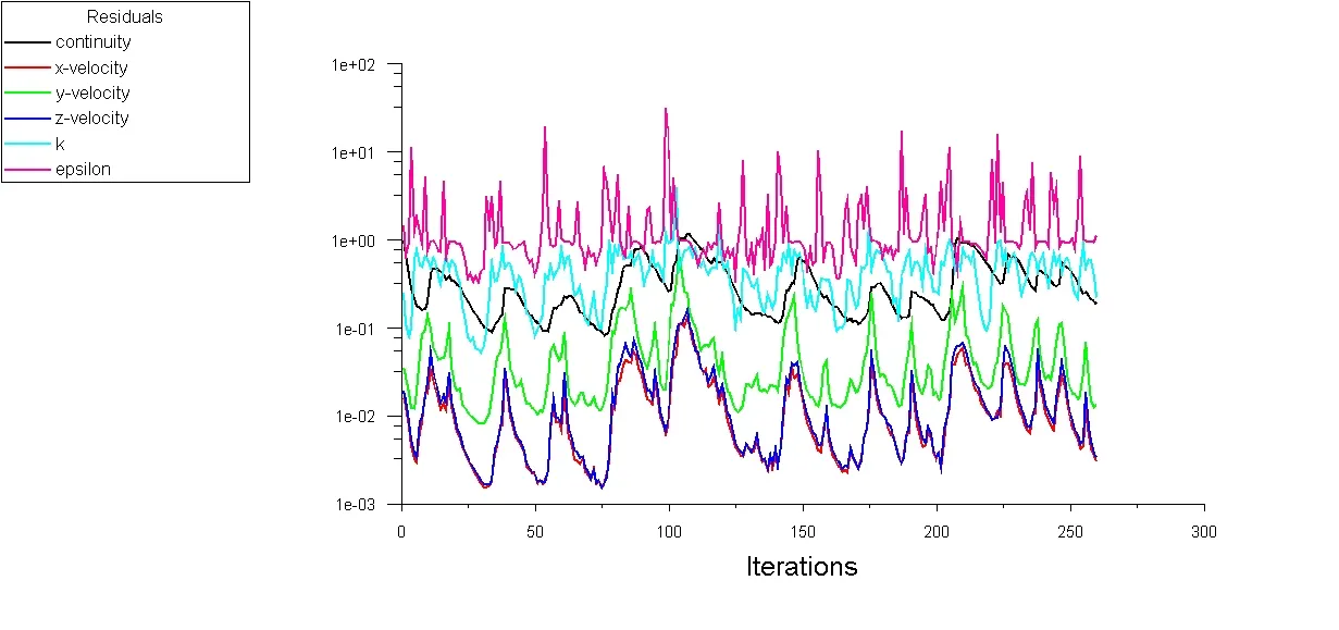
Figure 19, Convergence plot for 50% valve opening. Figure 20, Convergence plot for 60% valve opening.

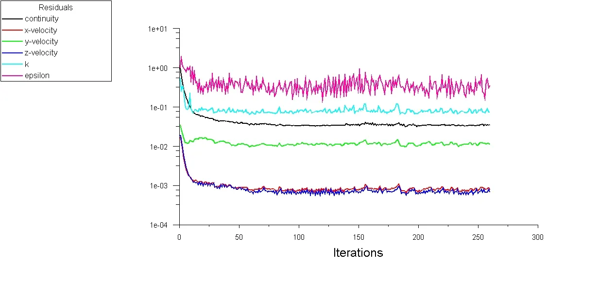
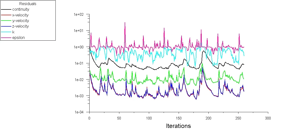
Figure 21, Convergence plot for 70% valve opening. Figure 22, Convergence plot for 80% valve opening.

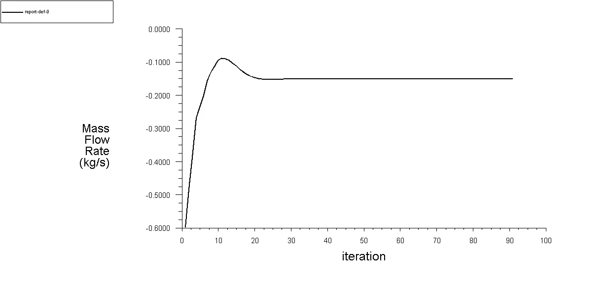
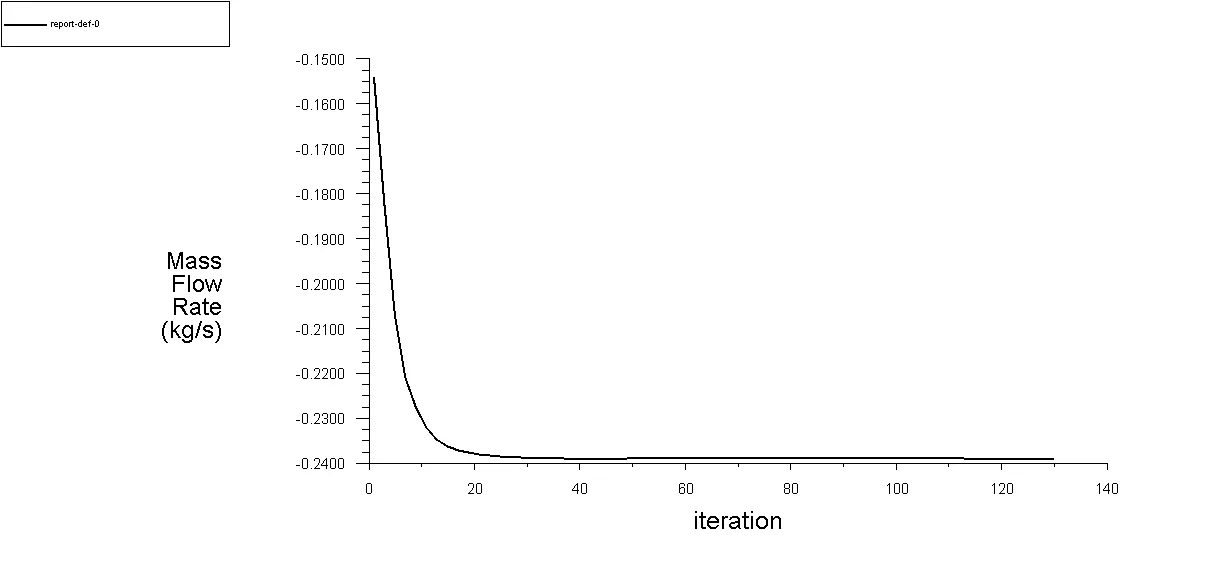
Figure 23, Mass flow at outlet for 10% valve opening. Figure 24, Mass flow at outlet for 20% valve opening.

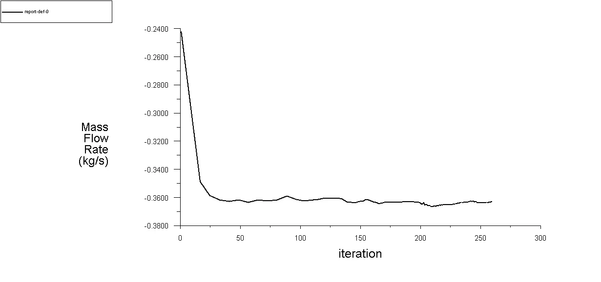
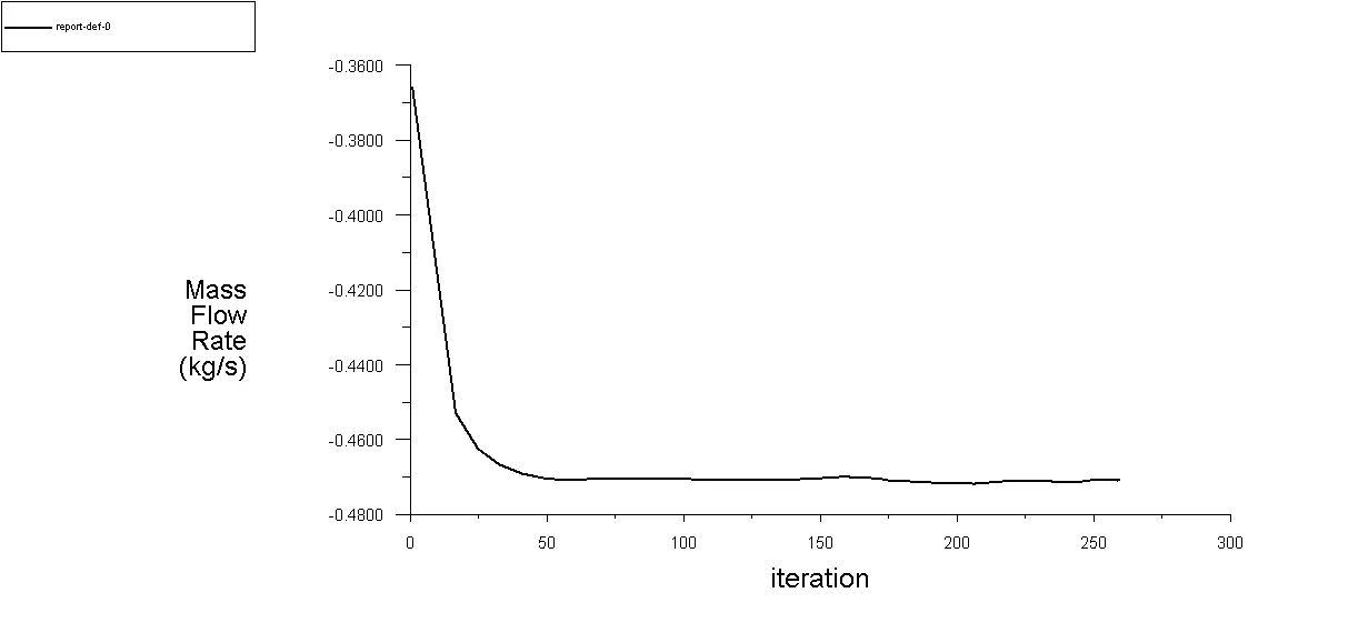
Figure 25, Mass flow at outlet for 30% valve opening. Figure 26, Mass flow at outlet for 40% valve opening.

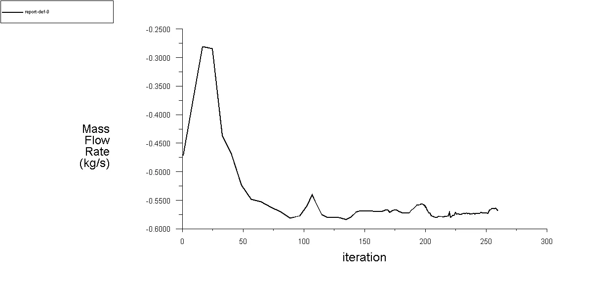
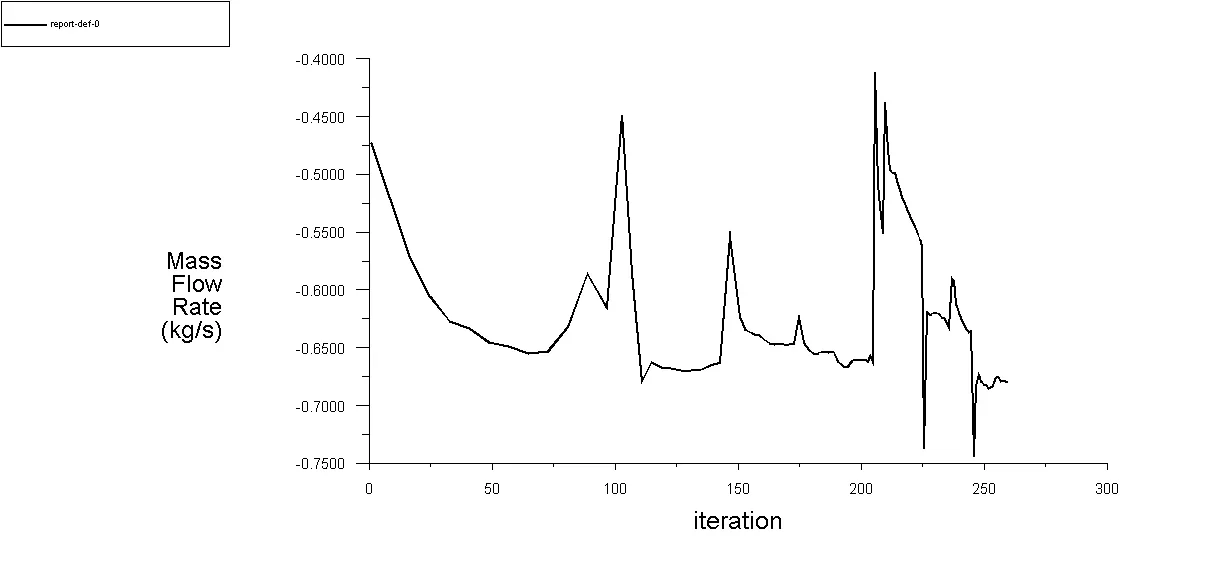
Figure 27, Mass flow at outlet for 50% valve opening. Figure 28, Mass flow at outlet for 60% valve opening.

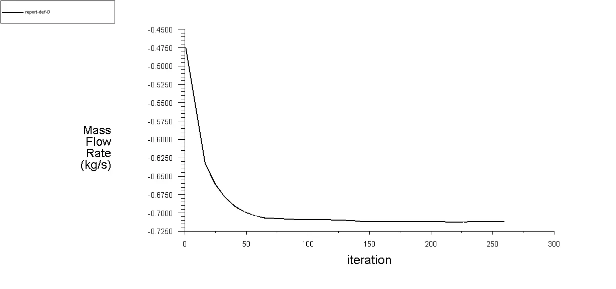
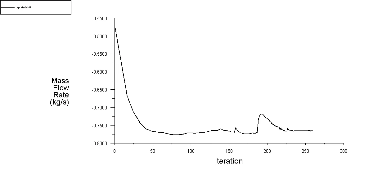
Figure 29, Mass flow at outlet for 70% valve opening. Figure 30, Mass flow at outlet for 80% valve opening.

Result are extracted from CFD Post and we can see that when valve Is only 10% open then the pressure is maximum at upstream and there be low pressure on downstream and due to that pressure drop is high.as the valve is continuous to open the pressure on the upstream is getting decreased due to lower restriction and then pressure drop is decreased. When flow opening is at our beyond 50% the pressure on both upstream and downstream getting nearly equal and pressure drop is low. When valve is 80% open the pressure is getting constant all along the upstream and downstream. The Figure from 31 to 38 shows the pressure contour on different valve opening.

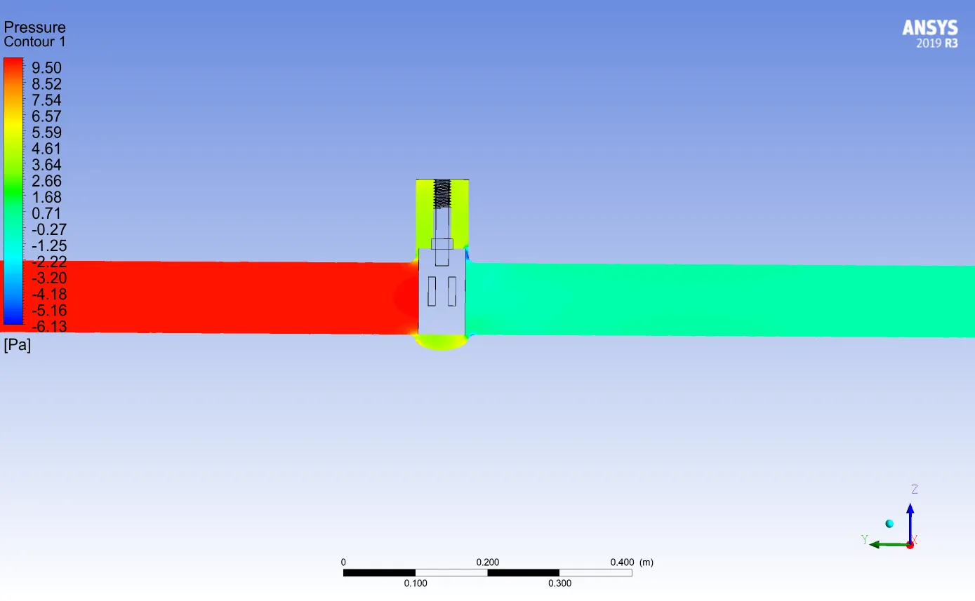
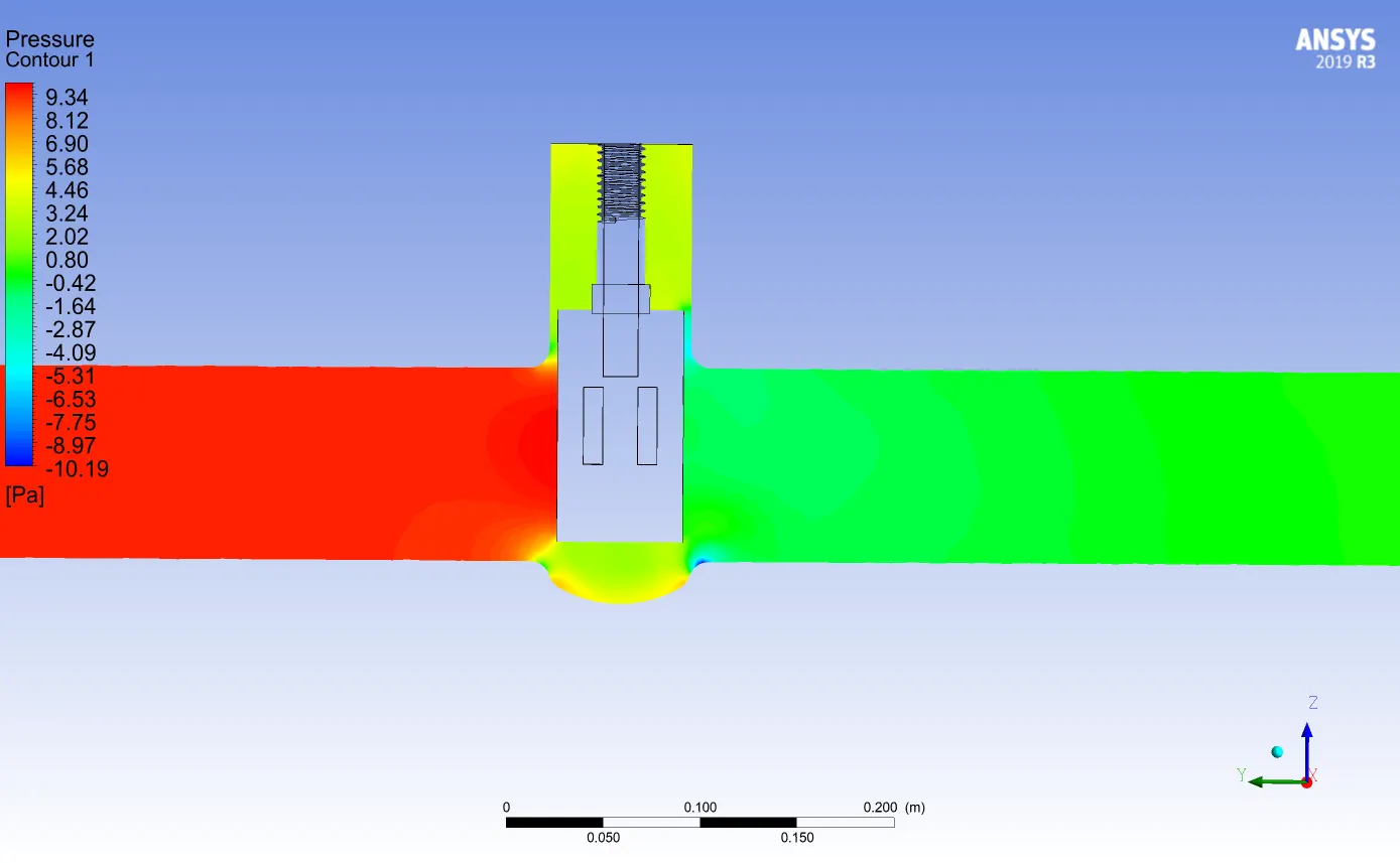
Figure 31,Pressure contour at 10% valve opening. Figure 32,Pressure contour at 20% valve opening.

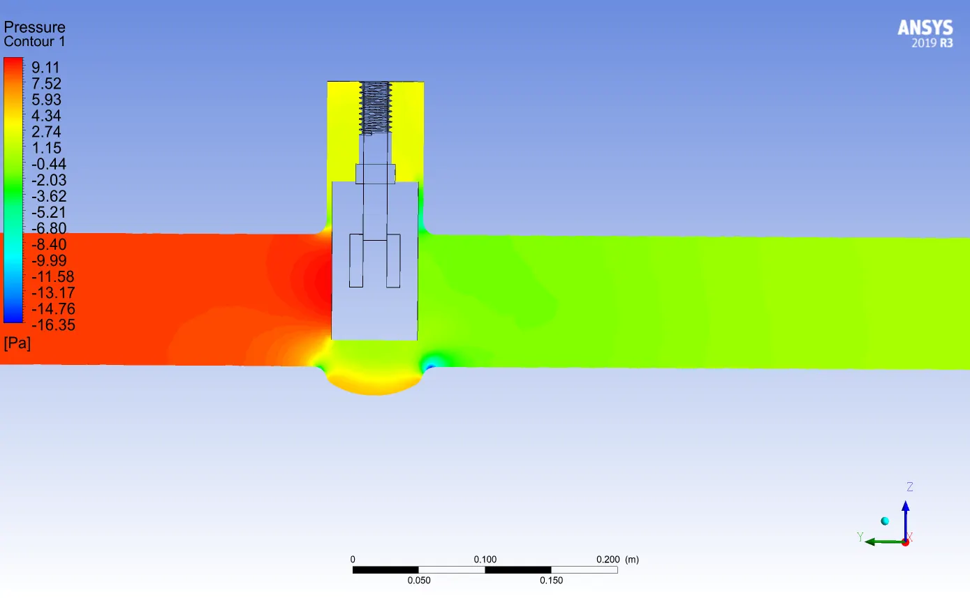
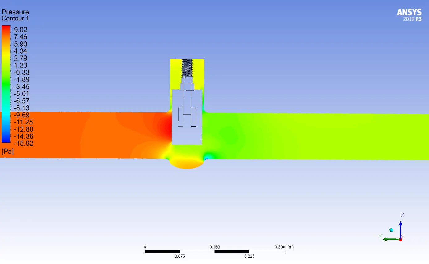
Figure 33,Pressure contour at 30% valve opening. Figure 34,Pressure contour at 40% valve opening.

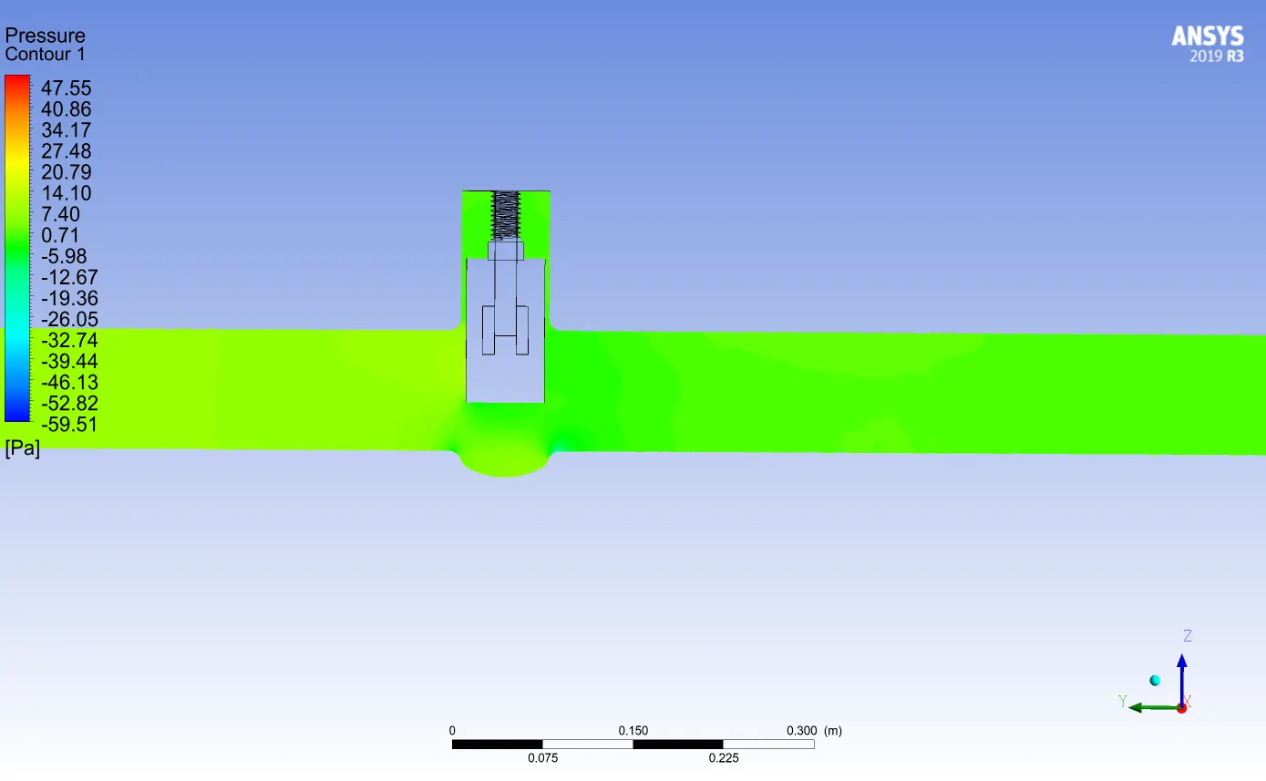
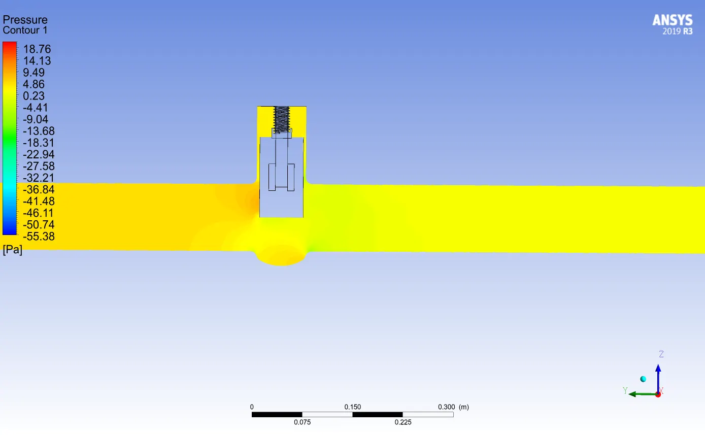
Figure 35,Pressure contour at 50% valve opening. Figure 36,Pressure contour at 60% valve opening.

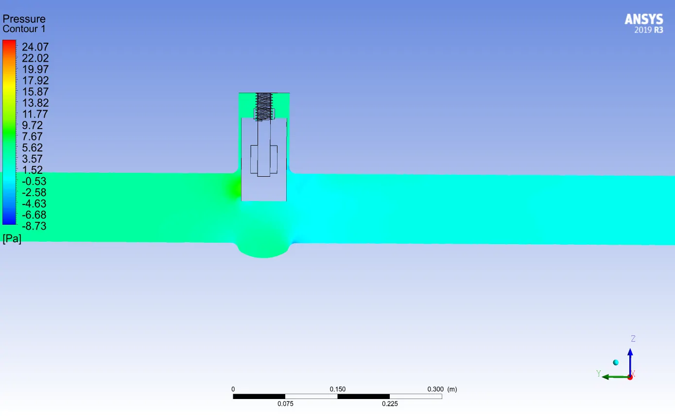
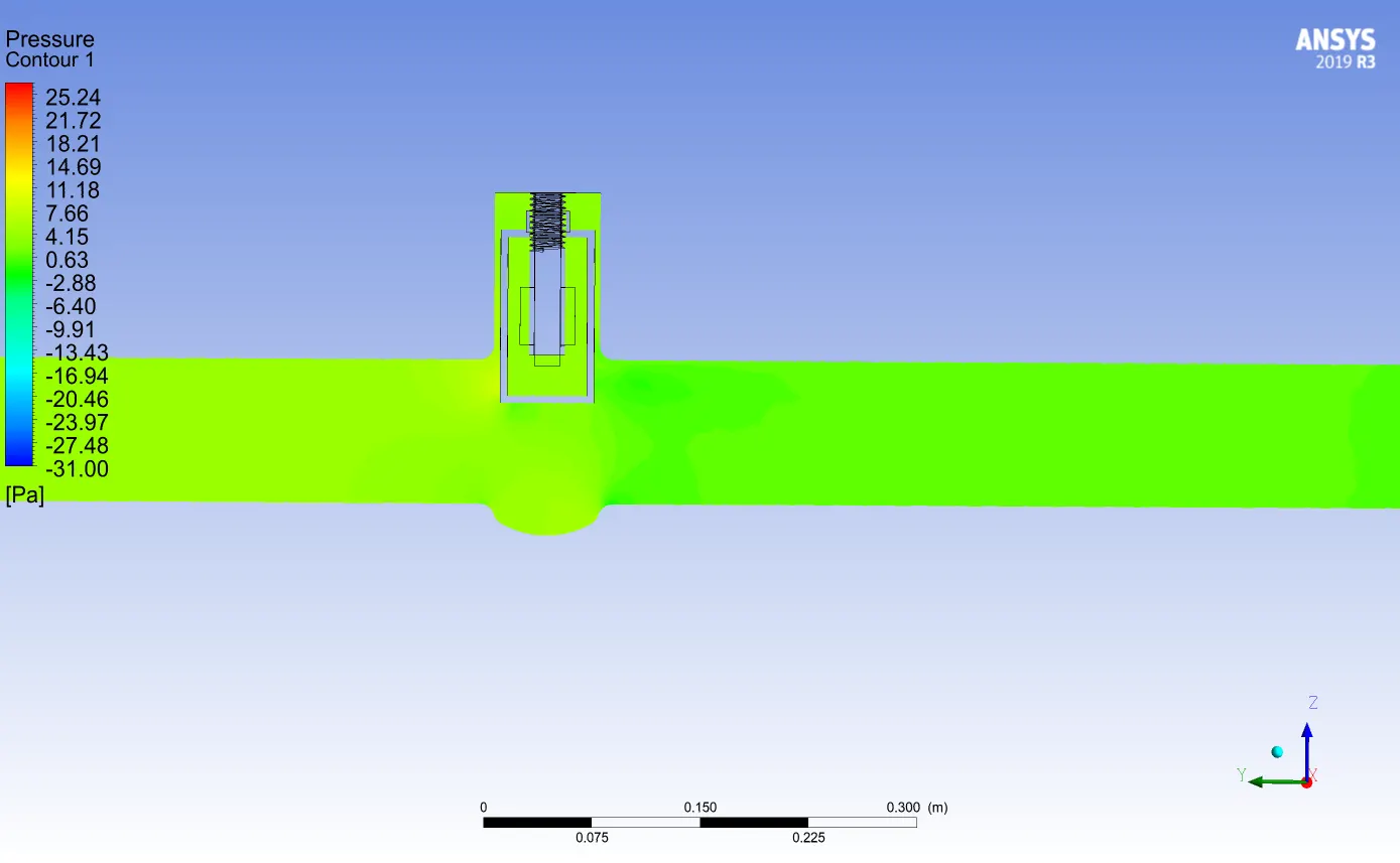
Figure 37,Pressure contour at 70% valve opening. Figure 38,Pressure contour at 80% valve opening.

Velocity on the restriction or narrow area is high due high pressure on upstream. Fluid leaves with maximum velocity when past the valve. And then there be some recirculation area on above portion of valve. but as the valve is continuous to open the velocity is maximum at flow restriction and then become normal to flow velocity. Below the valve stream there is region where the velocity is low due to recirculation. Figure from 39 to46 shows the velocity contour for different valve opening. Also from the stream line we can see that the fluid particle velocity suddenly increased when there is restriction , after that velocity become constant. Figure from 47 to 54 show the streamline contour at different flow opening.

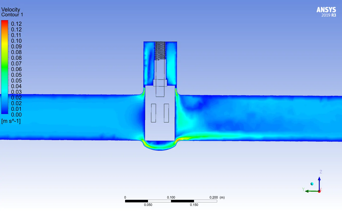
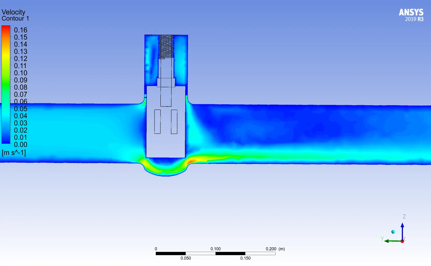
Figure 39, Velocity contour at 10% valve opening. Figure 40, Velocity contour at 20% valve opening.

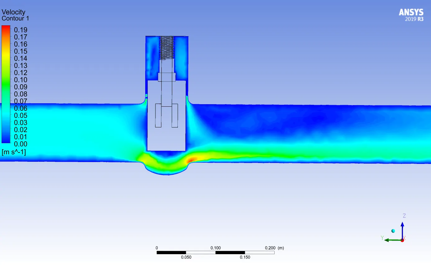
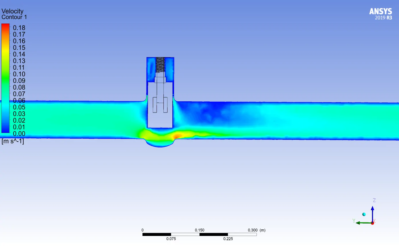
Figure 41, Velocity contour at 30% valve opening. Figure 42, Velocity contour at 40% valve opening.

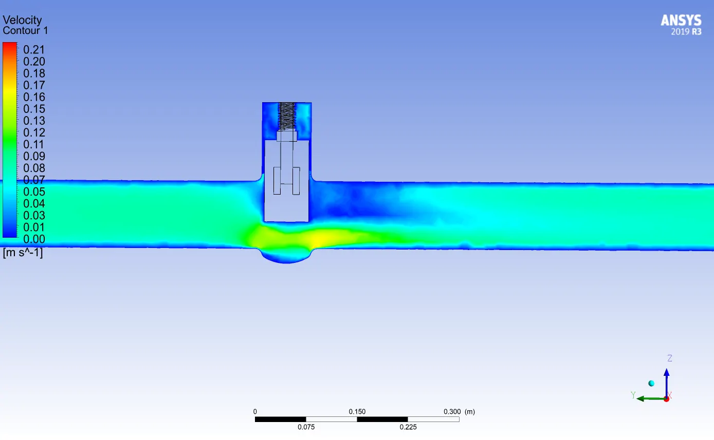
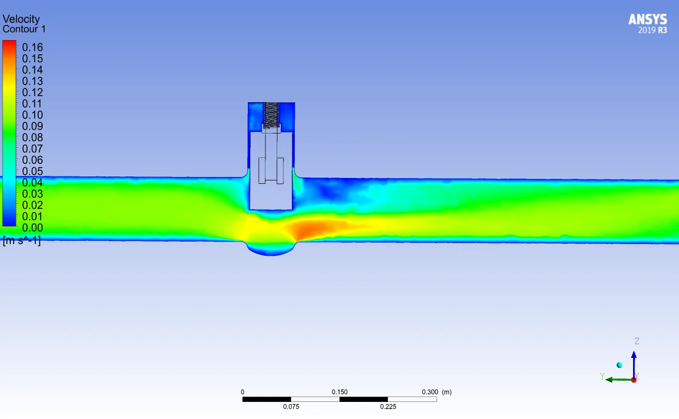
Figure 43, Velocity contour at 50% valve opening. Figure 44, Velocity contour at 60% valve opening.

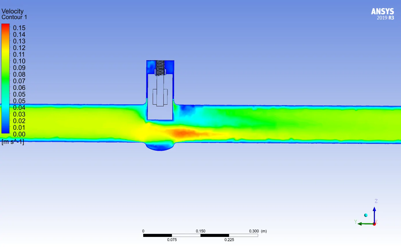
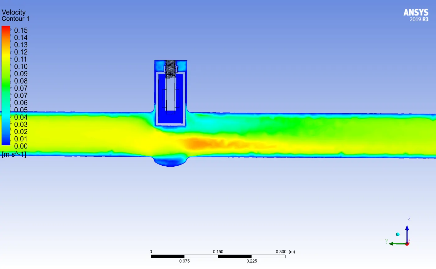
Figure 45, Velocity contour at 70% valve opening. Figure 46, Velocity contour at 80% valve opening.

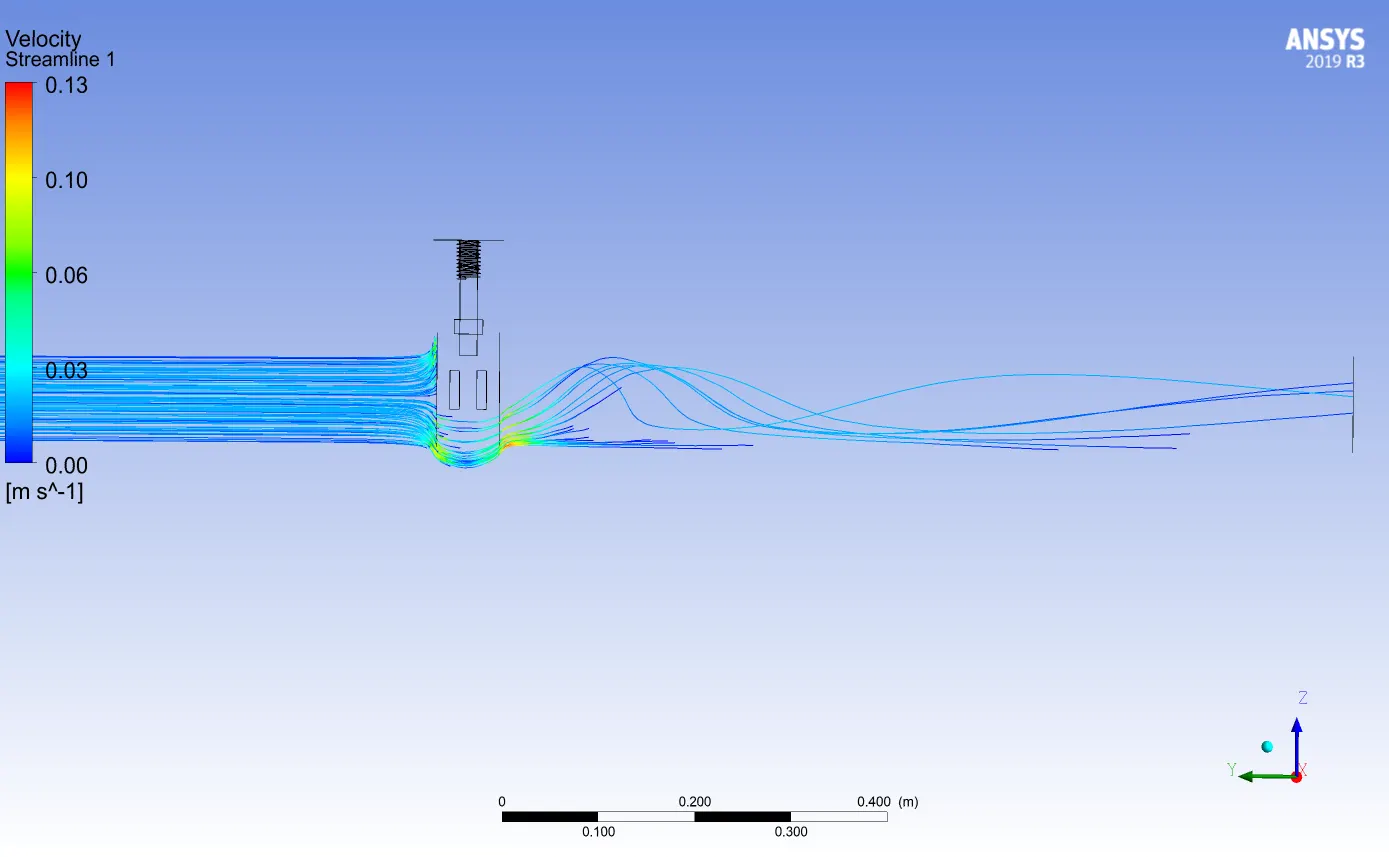
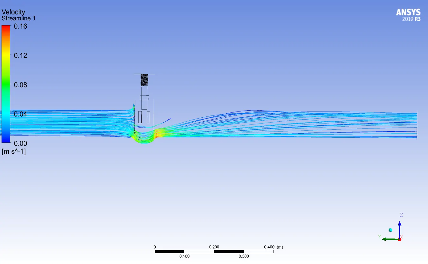
Figure 47,Streamline contour for 10% valve opening. Figure 48,Streamline contour for 20% valve opening.

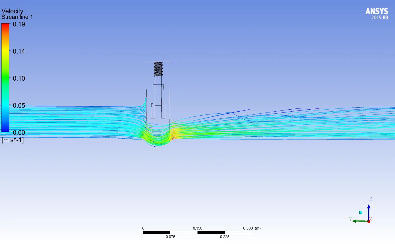
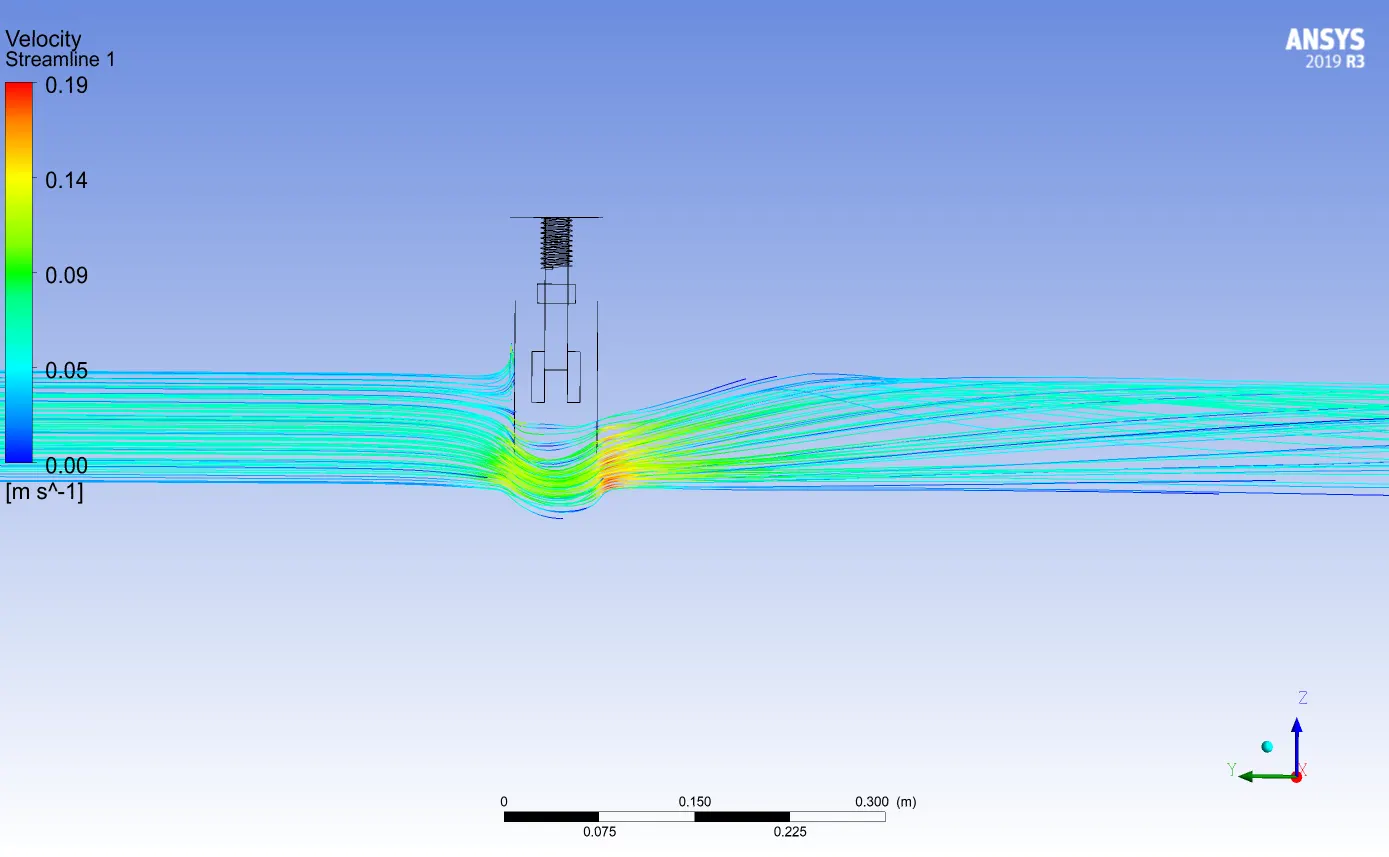
Figure 49,Streamline contour for 30% valve opening. Figure 50,Streamline contour for 40% valve opening.

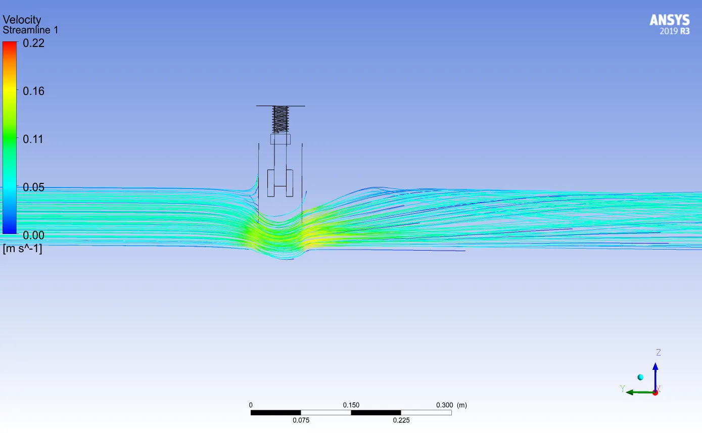
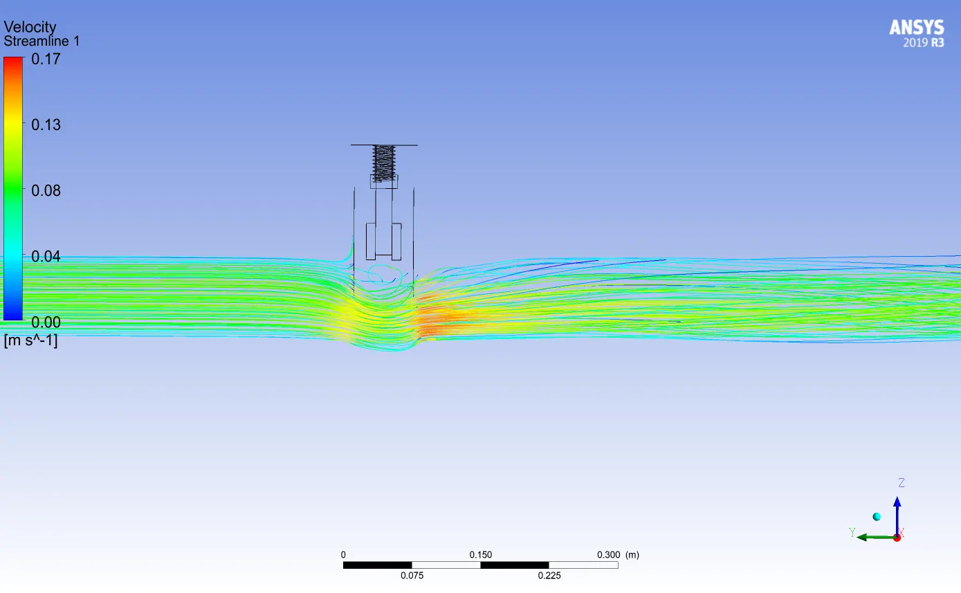
Figure 51,Streamline contour for 50% valve opening. Figure 52,Streamline contour for 60% valve opening.

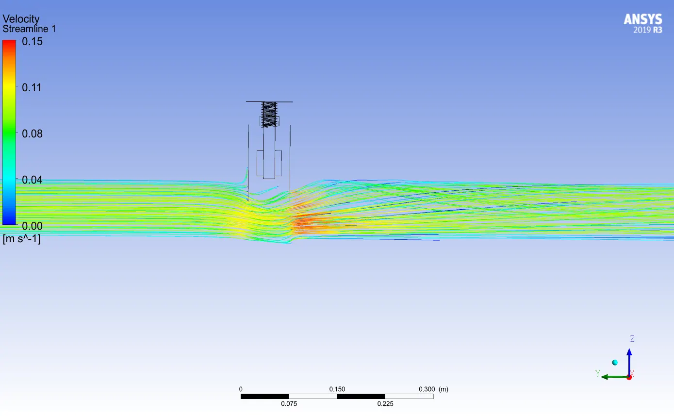
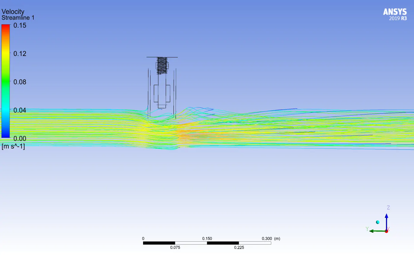
Figure 53,Streamline contour for 70% valve opening. Figure 54,Streamline contour for 80% valve opening.

To calculate the flow coefficient we choose above described formula and details are calculated from FLUENT. The data of pressure drop, flow coefficient and flow factor are shown in table 1.

Flow opening	Mass flow (m3/h)	Upstream pressure (Pascal)	Downstream pressure (Pascal)	Pressure drop	KV	CV
10%	0.537567854	9.689123182	-0.154248369	9.843371551	54.18279	62.6353
20%	0.861535684	9.176916705	-0.886008184	10.06292489	85.88378	99.28165
30%	1.300439591	7.883580172	-2.066565983	9.950146155	130.3693	150.707
40%	1.697990383	6.862030817	-2.012054927	8.874085744	180.2492	208.3681
50%	2.061109998	6.135221941	-1.751341122	7.886563063	232.0905	268.2966
60%	2.457319175	5.259372203	-2.078691714	7.338063917	286.8605	331.6108
70%	2.566235223	5.052878921	-0.302215539	5.35509446	350.6815	405.3878
80%	2.758316971	4.307129539	1.068177721	3.238951818	484.6653	560.2731

Table 1,

Figure 55 shows the plot of K_V and C_v against the different flow opening of valve. From the plot we can see that as the valve is opened the K_V and C_v are continuous to increased. Also from Figure 56 we can see that as the mass flow increases ,flow coefficient is also increased continuously. When the valve is 70% open the curve become more steep.

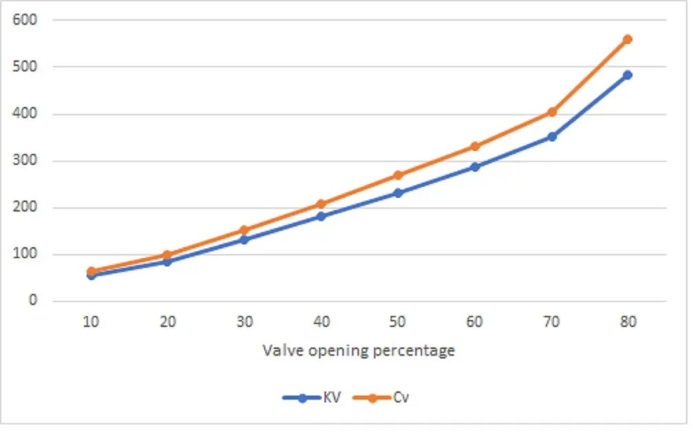
Figure 55, Plot for valve opening VS Kv and Cv.

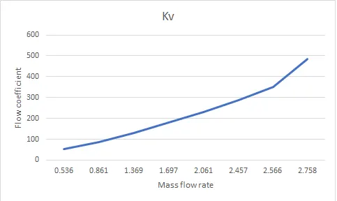
Figure 56, Plot for Flow coefficient VS mass flow rate.

Conclusion:-

The modelling methodology for the Flow Coefficient estimation for a Gate valve has been systematically investigated by considering flow parameters. The major focus of our simulation is to Carryout analysis of valves by using computer aided tools for the determination of flow coefficient, flow factor, mass flow at outlet and pressure drop. From the result we see that as the valve is continuous to open the flow coefficient and flow factor continuous to increased. from the simulation we have plotted pressure and velocity contour for different valve opening from 10% to 80%. When the opening is from 10% the velocity of fluid is maximum at the restriction and pressure at upstream is maximum than downstream resulting of higher pressure drop at low opening. As the restriction is decreased the flow pressure drop is decreased mass flow rate increased, flow coefficient and flow factor is increased in linear manner.