Gate Valve Parametric Study
JORGE LOZANO
Advanced CFD using ANSYS Fluent
Gate Valve Parametric Study
CHALLENGE FOR GATE VALVE SIMULATION:
For this challenge, you will have to perform a parametric study on the gate valve simulation by setting the opening from 10 % to 80%.
- Obtain the mass flow rates at the outlet for each design point.
- Calculate the flow coefficient and flow factor for each opening and plot the graph.
- Discuss the results of the mass flow rate and flow coefficient.
Theory
Parametric analysis in CFD
A low-cost, rapid way to analyze performance and optimize designs comes from what is called “parametric CFD analysis.” It includes five steps: problem definition, dimensional reduction, experimental design, management of CFD simulations, and metadata analysis. The metadata analysis stage may also include surrogate modeling, visualization, optimization, and sensitivity analysis.
Problem definition. For all designs, engineers must define requirements for the system, component, or process. For machines, requirements include the operating envelope of the equipment, which defines the range of conditions over which the device must operate safely.
Experimental design.
In this context, “experimental design” refers to the set of cases that the CFD code will run. The cases are selected to efficiently span the design space, with the goal of minimizing drag at cruise while retaining stability and control throughout the operating envelope. High-resolution CFD solutions of full aircraft configurations — especially landing configurations — are expensive, so the number of cases is limited. A space-filling design such as Latin hypercube (a statistical method), or one of its optimal variants, would probably be used to ensure coverage of the full range of each parameter.
Management of CFD simulations.
A key requirement for high-quality CFD solutions is that the grid-spacing be fine enough to resolve the dominant flow features. Ideally, a sufficiently fine grid would be used to resolve all these flow features to a high degree, but there are seldom enough computing resources to do this. Also, certain sub grid quantities, such as turbulence, are modeled, so no model is ideal for all flows. For this reason, CFD experts must evaluate the results to ensure assumptions aren’t violated.
Mastering CFD for engineering design.
Parametric CFD analysis has been shown to play a crucial role in the engineering design of fluid-dynamic devices. Without it, engineering methods can be costly and time consuming. By the time a project is complete, there could already by a more-efficient way to utilize the device. An understanding of the five stages of parametric CFD analysis gives users a better understanding of how a device behaves over its entire operating envelope and quickly produces better designs.
The flow coefficient of a device is a relative measure of its efficiency at allowing fluid flow. It describes the relationship between the pressure drop across an orifice valve or other assembly and the corresponding flow rate.
Mathematically the flow coefficient Cv (or flow-capacity rating of valve) can be expressed as:
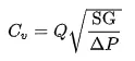
where:
- Q is the rate of flow (expressed in US gallons per minute),
- SG is the specific gravity of the fluid (for water = 1),
- ΔP is the pressure drop across the valve (expressed in psi).
The metric equivalent flow factor (Kv; commonly used in Europe and Asia) is calculated using metric units:
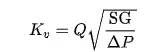
Where:
- Kv is the flow factor
- Q is the flowrate (expressed in cubic meters per hour),
- SG is the specific gravity of the fluid (for water = 1),
- ∆P is the differential pressure across the device (expressed in [bar]).
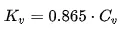
Kv can be calculated from Cv using the equation:
SIMULATION SET-UP
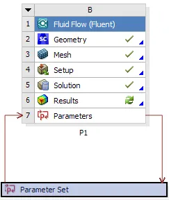
To perform simulations using Ansys/Fluent it’s desirable to have knowledge in the type of fluid model to adjust the condition of velocity inlet and the particles size, mesh characteristics, and the data postprocessing. For this case several simulations will be performed variating the initial conditions, duplicating several simulations and modifying the unique variables all these while using a parametric simulation which it’ll only have to be done once, by adding particular values into the cases, as in F.1.
F.1 Simulation Set up
Geometry
By using space claim software, the pipe fluid was obtained and extruded at the inlet and outlet length to obtain a wall defined flow due to the shear stress effect, as in F.2, the height of the valve gate is then parametrized to later on vary the dimension and perform a parametric simulation to see at different openings percentage the mass flow and pressure results.
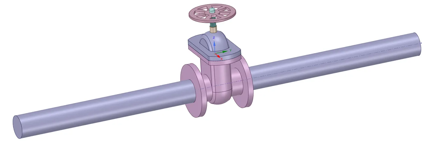
F.2 Pipe Geometry
Mesh
For these simulations one automatic mesh will be performed for every parametric geometry, having an element size of 5e-5 m and an inflation method around the walls. Considering a 512k element limit due to the educational software, the elements in both are approximately 450k elements for the mesh. Obtaining the quality with the skewness and orthogonality criteria, as both good mesh obtained.
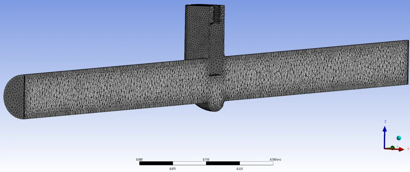
F.3 General mesh
Set up
The turbulence model selected is the K-epsilon method, due to the conditions and state of the model selected it will be a realizable K-epsilon model, with a scalable wall function, as F.4 having the constants and options selected.
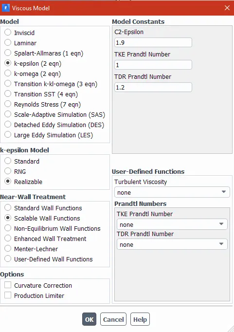
F.4 Turbulence model
The volume fluid material traveling along the pipe will be water, having its properties as in F.5.
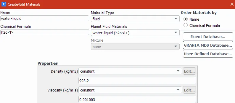
F.5 Materials
Results
F.6 to F.8 show the geometry variations from a 0 up to a 100 percentage of opening in the valve gate, obtaining the velocity and pressure in relation to the geometry variation, which is expected.
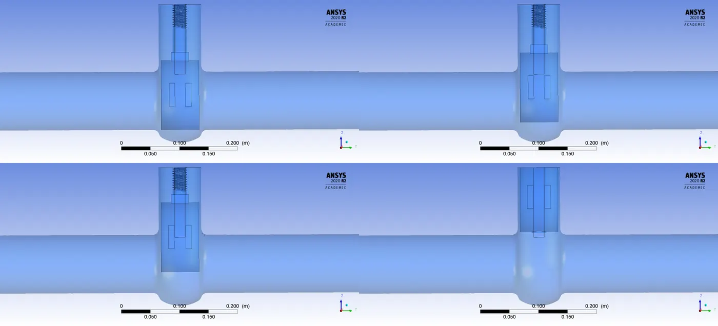
F.6 Geometry variations
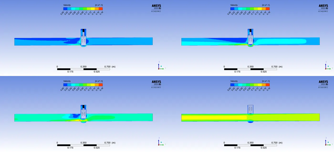
F.7 Velocity results
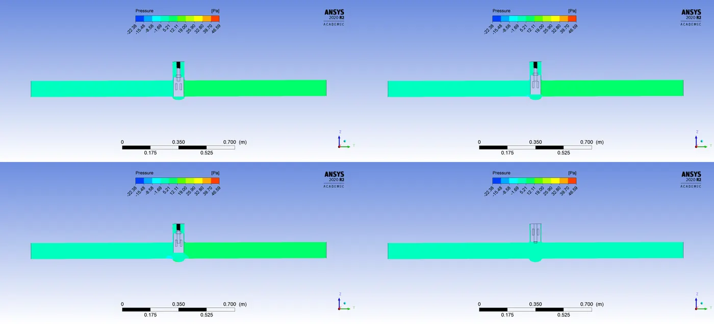
F.8 Pressure results
By using the parametric analysis, the software allows us have input and output automatic values, either manually adjusted or calculated, by having F.9 it represents exactly what fluent exports as parameters, that can be modified according to the conditions presented in the geometry and set up.

F.9 Input output parameters
To calculate the flow coefficient and flow factor, it’s important to determine the conversion of pressure and mass flow at the inlet and outlet, which determines the safety and performance of the valve.
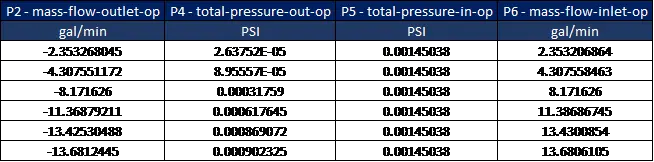
F.10 mass flow, pressure conversion
F.11 obtains the pressure difference and the specific gravity for water.
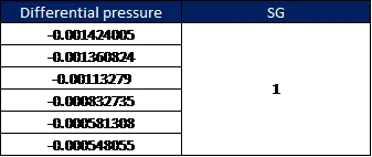
F.11 Differential pressure, and specific gravitation for water
The end results which will be graphed are the flow coefficient and flow factor, seen in F.12.
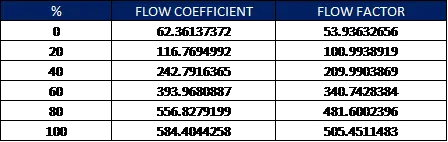
F.12 Flow value results
Conclusion
As conclusion in the results, the increase of the opening percentage, the flow factor and coefficient increases as the pressure difference decreases. By performing the parametric simulation, it was only needed to perform one set up with out any duplication and run automatically together, resulting in great computational time spent. F.13 shows the results obtained by the simulation in order to make decisions or compare to another valve geometry or type according to the needs and applications needed.
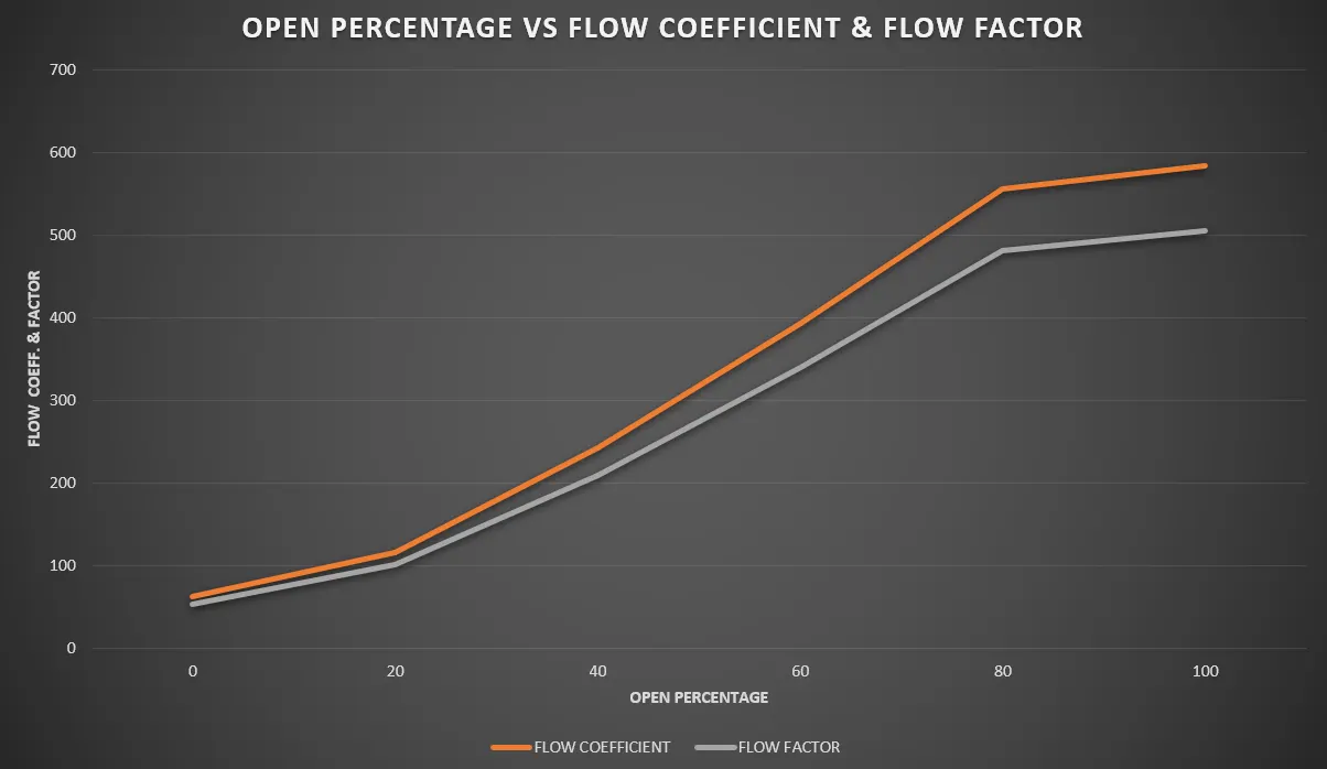
F.13 Opening percentage vs. flow coefficient and factor.
The following link has the workbench created at Ansys fluent:
https://drive.google.com/file/d/1CftOp4HK5on-kvk_UULZpbMZWk97-P3I/view?usp=sharing
References