FVM Literature Review
FDM :
In this method of discretization, we create mesh structure for the given geometry which provides us n no. of grid points. And then we solve the PDE in its Algebraic form at these grid points. We can expect correct answers as far as the grid points are linear along its axis. But as soon as it deviates, we have to apply a correction factor known as Variable Transformation method to get correct answers. The process is time consuming, but can be done with tedious coding procedure.
FVM :
In this method of discretization, the governing equations are solved in a discrete volumes, unlike FDM. The volume's shape is not assumed. It can be of any shape. The geometry then comprise of such small volumes and we solve the equations.
the procedure to do so is as follows : write the integral form of Governing equations ==> apply gauss divergence theorem ==> come up with suitable methods to calculate the flux terms.
Consider 1 dimensional state heat conduction equation with a source term. The source term is responsible for heat generation.
After discretizing the grid, the points we get are the centre of the volumes where the average quantities inside these volumes are stored. At first we say that the governing equation is valid at every point in our domains. Which then means it is also valid at the entire control volumes.
heat conduction equation : `del/(delx)(alpha *(delT)/(delx)) + S = 0`
If we multiply dv to 1st term and integrate it, `int(del)/(delx)(alpha*(delT)/(delx)*dv) + int S*dv = 0`
`therefore int_w^e del/(delx)(alpha*(delT)/(delx))* A*dx + int S*dv = 0`
`therefore [alpha*A*(delT)/(delx)]_w^e + barS*dv = 0`
`alpha_e*A*(delT)/(delx_e) - alpha_w*A*(delT)/(delx_w) + barS*dx = 0`
`alpha_e*A[(T_e-T_p)/(delx)] - alpha_w*A[(T_p - T_w)/(delx)] + barS*dv = 0`
the first term is heat flux which comes in the control volume and the second term is heat flux going out and the third is the source term.
Hence we can conclude that even in discretized form we can read the definition mathematically, unlike FDM.
FVM is said to conserve quantities better.
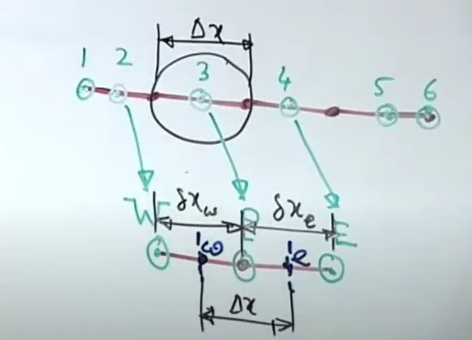
As per the image we consider the grid along x-axis and discretize it in several points (red points), and then observe a small section. We consider the centroid of the grid points as well which will be the centre of control volumes and posses the average values of the properties inside control volumes.
the distance between grid points is given as `dx` and distance between the neighbouring centroids is given as `delx`. According to the universal nomenclature we consider a point P and the grid point to the left as west W and to the right as east E. `delx_w and delx_e` are the distance between neighbouring centroids of point P. while solving the temperature for at point e and w as per figure we used neighbouring points. This is called as gradient scheme.
If `alpha_e` is the function of temperature, we need some kind of interpolation scheme to determine temperature at point e.
INTERPOLATION :
After integrating the governing differential equation over each sub-domain we consider a profile assumption for the dependent variable for evaluating above integrals. refer the figure below :
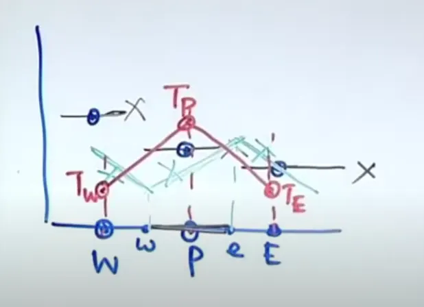
Here we have tried to consider different profiles to match the requirements so that we get a continious function at w and e points.
So the red line satisfies the condition because at point e and w the function is continious.
So the discretized form is given as : `alpha_e*[(T_e - T_p)/(delx_e)] - alpha_w*[(T_p - T_w)/(delx_w)] + S*dx = 0`
`therefore [(alpha_e)/(delx_e) + (alpha_w)/(delx_w)]*T_p = (alpha_e)/(delx_e)*T_e + (alpha_w)/(delx_w)*T_w + S*dx = 0`
it can be written as : `a_p*T_P = a_e*T_e + a_w*T_w + f`
where, `a_e = (alpha_e)/(delx_e) , a_w = (alpha_w)/(delx_w) , a_p = a_e + a_w, f = S*dx`
Need and different types of Interpolation schemes :
Linear/central differencing scheme : `phi_f` represents the physical quantities of the fluid at the face of the control volume. We use interpolation schemes to determine them. This scheme is same as linear interpolation. Instead of discretization schemes we can call it as face interpolation since we are keen to find the value of `phi_f` at every face , provided we know the value of neighbouring `phi` values at centroids.
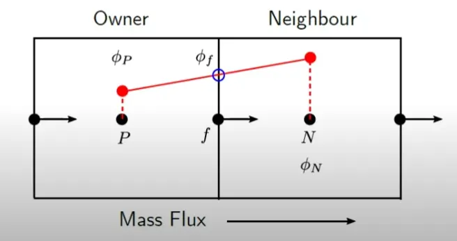
As per the figure, we can see that the value of `phi` changes linearly. So this scheme is second order accurate. Central differencing is used in diffusion term and it should never be used for convection term in RANS solver. It can be used for LES convection terms as greater accuracy is required there.
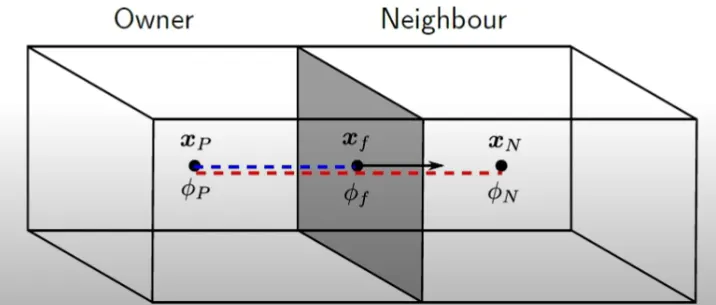
the formula for `phi_f` is given as : `phi_f` = `psi*phi_N + (1-psi)*phi_P` where `0<= psi <=1`
and `psi = abs(x_f-x_P)/abs(x_N-x_P)`
Upward differencing : It is not accurate but it is the most stable scheme for convection dominated flows. We can use it to generate an initial stable solution. So we first use it for initial approach and then we can switch to some other schemes.
`phi_f` = `phi_P` if the advection F>0 (mass flow out )
`phi_f` = `phi_N` if F<0 (mass flow in)
it is just the projection of the `phi_f` on the upcoming faces.The value between the cell centroid and face is constant hence it is first order accurate.
But in this scheme the discreet and defined structures are smeared out and that will lead to lose of resolution. So the physics of the flow will not be captured correctly.
Linear Upward differencing : It is a popular scheme in CFD. The scheme is also depends upon the mass flux. But here we have a gradient term to improve the accuracy of the interpolation.
`phi_f` = `phi_P` + `grad phi_P*r` if F > 0
`phi_f` = `phi_N` + `grad phi_N*r` if F < 0
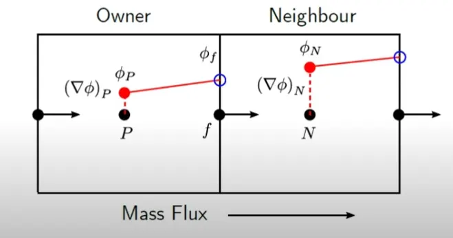
Now here the projection is no longer horizontal but we use gradient of `phi` to improve the accuracy. This is second order accurate because we see a linear variation from one cell's centroid to the next cell's face. It is popular for convection term.
This scheme is slightly unstable because we are getting a higher value of `phi` at face than at the centroid. This will lead to oscillations in our solutions which will lead to instability. So we have to bring the value of `phi` down and we do that by limiting the gradient. This way the `phi` values at the face wont be greater than `phi`at centroid.
The modification we propose is that : `phi_f = phi_P + psi*(gradphi)_P *r` where `0<=psi<=1` we introduce a limiter which range between 0 to 1.
Advanced discretization schemes : We can start with linear/central differencing for accuracy and then switch to upwind differencing for stability.
it is given as : `phi_f = psi*phi_(UD) + (1-psi)*phi_(CD)`
`psi` is a blending function to switch between schemes. If we have `psi` as 0, then we have central differencing and if 1 then upward differencing.
Flux limiters : When we calculate gradients, we need to have those values bounded. In shock flow problems, there is huge discontinuity, so the gradients can be of huge values, hence we have flux limiters.