linear and cubic polynomial fit for the cp data
AIM:- To Write code to fit a linear and cubic polynomial for the Cp data.
INTRODUCTION:-
Curve fitting is one of the most powerful and most widely used analysis tools in Origin. Curve fitting examines the relationship between one or more predictors (independent variables) and a response variable (dependent variable), with the goal of defining a "best fit" model of the relationship.
Origin provides tools for linear, polynomial, and nonlinear curve fitting along with validation and goodness-of-fit tests. You can summarize and present your results with customized fitting reports.
Interpolation:-Interpolation is a method of estimating values between known data points. Use interpolation to smooth observed data, fill in missing data, and make predictions.
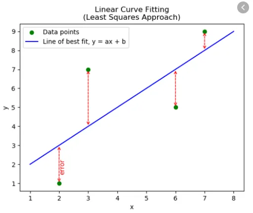
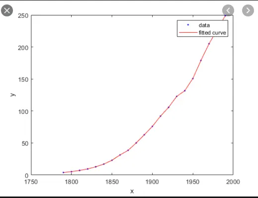
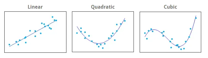
">regression analysis, curve fitting is the process of specifying the model that provides the best fit to the specific curves in your dataset. Curved relationships between variables are not as straightforward to fit and interpret as linear relationships.
For linear relationships, as you increase the Predictor variables
">independent variable by one unit, the Mean
">mean of the Response variables
">dependent variable always changes by a specific amount. This relationship holds true regardless of where you are in the observation space.
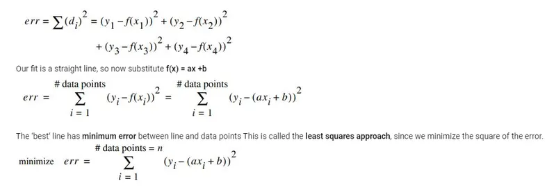
Positive or negative error have the same value (data point is above or below the line Weight greater errors more heavily (we can do both of these things by squaring the distance)
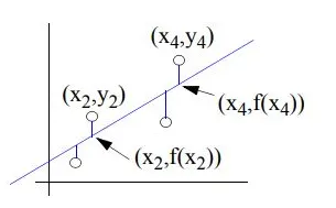
denote data values as (x, y)
denote points on the fitted line as (x, f(x))
sum the error at the four data points
Objective:
1)To fit a linear and cubic polynomial for the Cp data.
2)Plot the linear and cubic fit curves along with the raw data points.
3)Write a code to show split-wise method.
MATLAB PROGRAMME:-
1) LINEAR AND CUBIC FIT
close all
clear all
clc

cp_data=load('data') %loading of file
temp=cp_data(:,1)
cp=cp_data(:,2)
% for linear polynomial
co_eff1=polyfit(temp,cp,1)
%calculated cp
c_cp1=polyval(co_eff1,temp)
%plotting
figure(1)
plot(cp,temp,'linewidth',3,'color','r')
hold on
 plot(c_cp1,temp,'linewidth',3,'color','b')
xlabel('cp,c_cp1')
ylabel('temp')
legend('cp','c_cp1')
%testing the fitness
MEAN1=mean(c_cp1)
SSR1=sum((c_cp1-MEAN1).^2);
SSE1=sum((cp-c_cp1).^2);

SST1=SSR1+SSE1
R_SQUARE1=SSR1/SST1

%for cubic polynomial
co_eff2=polyfit(temp,cp,3) %polyfit for generating the coefficient
%calculated cp
c_cp2=polyval(co_eff2,temp)
%plotting
figure(2)
plot(cp,temp,'linewidth',3,'color','r')
hold on
 plot(c_cp2,temp,'linewidth',3,'color','b')
xlabel('cp,c_cp2')
ylabel('temp')
legend('cp','c_cp2')
%testing the fitness
MEAN2=mean(c_cp2)
SSR2=sum((c_cp2-MEAN2).^2);
SSE2=sum((cp-c_cp2).^2);

SST2=SSR2+SSE2
R_SQUARE2=SSR2/SST2
2)
close all
clear all
clc

cp_data=load('data')
temp=cp_data(:,1)
cp=cp_data(:,2)
% splitting original temp data
T1=cp_data(1:800,1)
T2=cp_data(800:1600,1)
T3=cp_data(1600:2400,1)
T4=cp_data(2400:3200,1)
% splitting original cp_data
cp1=cp_data(1:800,2)
cp2=cp_data(800:1600,2)
cp3=cp_data(1600:2400,2)
cp4=cp_data(2400:3200,2)

%% now using T1 and cp1
co_eff=polyfit(T1,cp1,4)

c_cp1=polyval(co_eff,T1)
%plotting
figure(1)
plot(cp1,T1,'linewidth',3,'color','r')
hold on
plot(c_cp1,T1,'linewidth',3,'color','b')
xlabel('cp,c_cp')
ylabel('T1')
legend('cp','c_cp')

%%NOW checking the fitness of the curve
MEAN1=mean(c_cp1)
SSR1=sum((c_cp1-MEAN1).^2);
SSE1=sum((cp1-c_cp1).^2);

SST1=SSR1+SSE1
R_SQUARE1=SSR1/SST1


% now using T2 and cp2
co_eff=polyfit(T2,cp2,3)

c_cp2=polyval(co_eff,T2)
%plotting
figure(2)
plot(cp2,T2,'linewidth',3,'color','r')
hold on
plot(c_cp2,T2,'linewidth',3,'color','b')
xlabel('cp2,c_cp2')
ylabel('T1')
legend('cp2','c_cp2')

%NOW checking the fitness of the curve
MEAN2=mean(c_cp2)
SSR2=sum((c_cp2-MEAN2).^2);
SSE2=sum((cp2-c_cp2).^2);

SST2=SSR2+SSE2
R_SQUARE2=SSR2/SST2


%% now using T3 and cp3
co_eff=polyfit(T3,cp3,2)

c_cp3=polyval(co_eff,T3)
%plotting
figure(3)
plot(cp3,T3,'linewidth',3,'color','r')
hold on
plot(c_cp3,T3,'linewidth',3,'color','b')
xlabel('cp3,c_cp3')
ylabel('T3')
legend('cp3','c_cp3')

%%NOW checking the fitness of the curve
MEAN3=mean(c_cp3)
SSR3=sum((c_cp3-MEAN3).^2);
SSE3=sum((cp3-c_cp3).^2);

SST3=SSR3+SSE3
R_SQUARE3=SSR3/SST3


%% now using T4 and cp4
co_eff=polyfit(T4,cp4,3)

c_cp4=polyval(co_eff,T4)
%plotting
figure(4)
plot(cp4,T4,'linewidth',3,'color','r')
hold on
plot(c_cp4,T4,'linewidth',3,'color','b')
xlabel('cp4,c_cp4')
ylabel('T4')
legend('cp4','c_cp4')

%%NOW checking the fitness of the curve
MEAN4=mean(c_cp4)
SSR4=sum((c_cp4-MEAN4).^2);
SSE4=sum((cp4-c_cp4).^2);

SST4=SSR4+SSE4
R_SQUARE4=SSR4/SST4
STEPS INVOLVED IN CURVE FITTING:-
1)Load the data from the data file.
2)Extract the co-efficient of the polynomial for linear and cubic fit using polyfit command.
3)Store the predicted value of linear and cubic polynomial using polyval command.
4) Make a plot to compare raw data points with predicted data and see if the curve fits.
5) Make plot for both linear and cubic polynomial. s.
6) Compute the value of SSE, R_square, RMSE.
7) Use these calculated values compare the goodness of fit for linear and cubic polynomials
8) If the value of R_square is greater than then the fitness of the curve is assumed to be good
.
GOVERNING EQUATIONS:
1)Sum of squared errors (SSE) SSE = E(Y(i) — f(x(i)))
Where, f(x(i)) = Mean
2) R-square
'R"2 = (SSR)/(SST)'
Where,
SSR = sum of square of regression, which is square of the difference between the value of the fitting function at a given point and the arithmetic mean of data set.
If y = f(x) is the fit curve then the SSR is defined as,
SSR = E(f(x(i)) — Mean)
SSE = E(Y(i) — f(x(i)))
Now, SST is given by SST = SSR + SSE This give us the value of R-square
FOR SPLITWISE METHOD
temp is divided into 4 parts and cp is also divided into 4 ,individual 4 section result has been taken out with plots
OUTPUT:-
PLOT FOR LINEAR CURVE:-
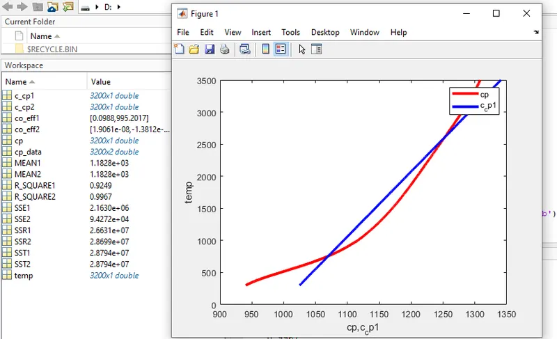
R_SQUARE=0.9249
PLOT FOR CUBIC
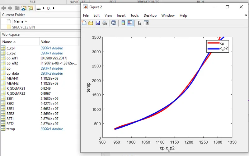
RSQUARE:-0.9967
PLOTS FOR SPLITWISE METHOD
1) FOR T1 AND cp1
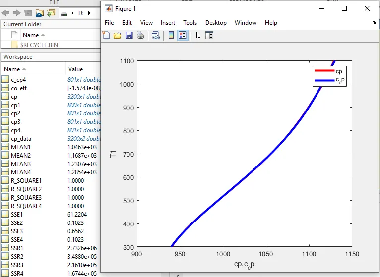
R_SQUARE=1.0000
2) FOR T2 AND cp2
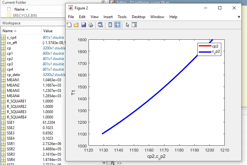
R_SQUARE:-1.0000
3) T3 and cp3
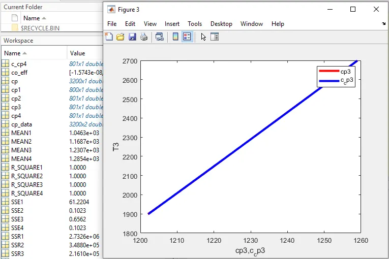
R_SQUARE:-1.0000
4)T4 AND cp4
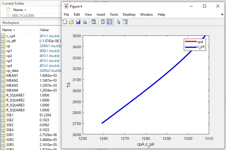
R_SQUARE:-1.0000
Based on the research, answer for following questions are:
1)How to make a curve fit perfectly?
Ans:- to make a fit there are no. method can be used, like -Split-Wise Method -Different Polynomial Order -One Polynomial for one Temperature Range and Different Polynomial Order for Different Temperature Range.
2)How to get the best fit?
Ans:- Upon finding a curve which satisfy the data there are 4 quantities which help us measure the goodness of fit. The sum of Square due to Error (SSE) R-square Adjusted R-square Root mean Squared Error (RMSE)
3) what could be done to improve the cubic fit?
Ans:- We can use use the Split-Wise Method and Fitted the curve by spliting the curve over the actual data. we can make a program which ask the user of number of split, so that best fit after split can be made.