Analyse the Transient Flow Simulation over a cylinder with the different Reynold's number and establishing Transient flow for Pressure and Velocity profiles using Solidworks

OBJECTIVE :- To simulate a Transient flow over a cylinder for various Reynolds number establishing a transient flow for Pressure and Velocity profiles using SolidWorks

COMPUTATIONAL FLUID DYNAMICS (CFD) :-

Computational fluid dynamics (CFD) is a branch of fluid mechanics that uses numerical analysis and data structures to analyze and solve problems that involve fluid flows. Computers are used to perform the calculations required to simulate the free-stream flow of the fluid, and the interaction of the fluid (liquids and gases) with surfaces defined by boundary conditions. With high-speed supercomputers, better solutions can be achieved, and are often required to solve the largest and most complex problems. Ongoing research yields software that improves the accuracy and speed of complex simulation scenarios such as transonic or turbulent flows. Initial validation of such software is typically performed using experimental apparatus such as wind tunnels. In addition, previously performed analytical or empirical analysis of a particular problem can be used for comparison. A final validation is often performed using full-scale testing, such as flight tests.

CFD is applied to a wide range of research and engineering problems in many fields of study and industries, including aerodynamics and aerospace analysis, weather simulation, natural science and environmental engineering, industrial system design and analysis, biological engineering, fluid flows and heat transfer, and engine and combustion analysis.

Methodology:-

In all of these approaches the same basic procedure is followed.

During preprocessing

• The geometry and physical bounds of the problem can be defined using computer aided design (CAD). From there, data can be suitably processed (cleaned-up) and the fluid volume (or fluid domain) is extracted.
• The volume occupied by the fluid is divided into discrete cells (the mesh). The mesh may be uniform or non-uniform, structured or unstructured, consisting of a combination of hexahedral, tetrahedral, prismatic, pyramidal or polyhedral elements.
• The physical modeling is defined – for example, the equations of fluid motion + enthalpy + radiation + species conservation
• Boundary conditions are defined. This involves specifying the fluid behaviour and properties at all bounding surfaces of the fluid domain. For transient problems, the initial conditions are also defined.

• The simulation is started and the equations are solved iteratively as a steady-state or transient.
• Finally a postprocessor is used for the analysis and visualization of the resulting solution.

Reynold's Number:

In this project Reynold's Number (Dimensionless quantity in fluid dynamics) is used to predict flow patterns in different types of simulations and transition from laminar to turbulent flow.

While Reynold's Number 100 & 1000 fall into Laminar category, 10000 belongs to the Turbulent flow

The formula for calculating Reynold's Number is given below:

Reynolds number, Re = (rho * D * flow speed) / mu

where, D = cylinder diameter

mu = dynamic viscosity

rho = density

flow speed = inlet velocity or pressure

Air is taken as medium

Density of air = 1.225 kg/m^3

Dynamic viscosity of air = 1.81*10^-5 kg/(m.s)

The above picture represents the velocity of a flow at different levels causing various pressure/velocity differences. The region behind the flow of cylinder is called "Wake region" and point at start and end points of the cylinder in the direction of flow is called "Stagnation point". The Boundary layer separation takes place along the cylinder flow.

A sample of the flows behavior over a cylinder when the Reynolds number is increased is given below.

Laminar flow Occurs when Reynold’s number Re< 2000.

In laminar flow velocity increases gradually from zero at the boundary to Maximum at the center. Laminar flow is regular and smooth and velocity at any point practically remains constant in magnitude & direction. Therefore, the flow is also known as stream Line flow.

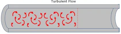
Turbulent flow occurs when Reynolds number above 4000.

In the turbulent flow the fluid flow at higher flow rates, the streamlines are not steady and straight and the flow is not laminar. Flow is very much disorder and there will be violent mixing.

Transitional Flow

In this, the condition is neither the laminar nor turbulent. It is intermittently turbulent flow. The stream lines get disturbed a little.
This type of flow occurs when 2000< Re < 4000.

GOVERNING EQUATIONS :-

Dynamic viscosity Ns/m^2 (also known as absolute viscosity) is the measurement of the fluid’s internal resistance to flow while kinematic viscosity...m^2/s refers to the ratio of dynamic viscosity to density.

Kinematic Viscosity of Air @293K = 1.516*10^-5 m^2/s

CALCULATION :-

CALCULATIONS

Re=[V.D]/v
  =[10*0.05]/1.516*10^-5
  =‭32,981

So, The 3 different inputs for Reynolds Numbers with diff factors are as follows,

Increased Factor       Re        Velocity

Obtained               32981     10 (given)
+20%                   39578     12
+40%                   46173     14
+100%                  65962     20

To calculate flow through time for 4 different cases,

Velocity=[Distance/Time] ie; Time=[Distance/Velocity]

Case 1
T = 0.54/10 = 0.054s

Case2
T = 0.54/12 = 0.045s

Case3
T = 0.54/14 = 0.0385s

Case4
T = 0.54/20 = 0.027s

Considering end time is 2 times the flow through time

T1 = 0.108s
T2 = 0.09s
T3 = 0.0771s
T4 = 0.054s

PROCEDURE :-

• Open SolidWorks and Create a new Part file.
• Sketch a Cylinder of diameter 0.03m and extrude it to length 0.06m which will give us the following figure.

• Save the Sketch and click Wizard under Flow Simulation tab.
• The parameters are set as Time dependent flow, air as our fluid and velocity is set at x axis (i.e 10, 12, 14 & 20 m/s for varying Reynold's number percentage such as 0, 20, 40 & 100).

• Global Mesh can be edited to make the result finer by increasing the levels of intial mesh.
• Now Run the simulation which will load the results.
• Under Results, create a Cut plot for both Pressure & Velocity.

• Finally, the animation is created for both the plots with respective parameters using animation wizard option.
• And click on scenerio option in animation wizard.
• Evaluate the Results with the obtained Plots.

RESULTS :-

Cut Plots for Velocity and Pressure and its TRANSIENT ANIMATIONS :-

SIMULATION @10 m/sec -

SIMULATION @12 m/sec -

SIMULATION @14 m/sec -

SIMULATION @20 m/sec -

CONCLUSION :-

From the above study we can conclude that

• It is higher in the region above & below the cylinder facing the flow while the velocity at back gradually decreases creating a Wake region in the boundary layer.
• Due to Stagnation pressure at the front of the cylinder facing the flow, it has higher pressure while minimum at the back of the cylinder..
• Due to the cylindrical structure, there exists an Maximum Velocity region pointing radially outwards indicated by Red Colour in the Plots.
• The other side of the Cylinder towards exit of the flow experiences very low velocity range due to presence of obstruction indicated by Greenish Blue Colour in the Velocity Plots.
• With increase in the Reynolds Number, the inlet Velocity Increases and puts same effect on the walls of the Cylinder, only the extent of the Flow along with range of obstruction for the flow velocity changes.