Performing optimization of the stalagmite function using Genetic Algorithm and Calculate global maxima
AIM:- To optimize the stalagmite function using Genetic Algorithm.
Objective:-
- To Plot stalagmite function.
- To calculate the global maxima of a stalagmite function using 3 statistical cases.
Genetic Algorithm(ga):-
A genetic algorithm (GA) is a method for solving both constrained and unconstrained optimization problems based on a natural selection process that mimics biological evolution. The algorithm repeatedly modifies a population of individual solutions. At each step, the genetic algorithm randomly selects individuals from the current population and uses them as parents to produce the children for the next generation. Over successive generations, the population "evolves" toward an optimal solution.
You can apply the genetic algorithm to solve problems that are not well suited for standard optimization algorithms, including problems in which the objective function is discontinuous, nondifferentiable, stochastic, or highly nonlinear.
The genetic algorithm differs from a classical, derivative-based, optimization algorithm in two main ways, as summarized in the following table.
| Classical Algorithm | Genetic Algorithm |
|---|---|
| Generates a single point at each iteration. The sequence of points approaches an optimal solution. | Generates a population of points at each iteration. The best point in the population approaches an optimal solution. |
| Selects the next point in the sequence by a deterministic computation. | Selects the next population by computation which uses random number generators. |
The following outline summarizes how the genetic algorithm works:
-
The algorithm begins by creating a random initial population.
-
The algorithm then creates a sequence of new populations. At each step, the algorithm uses the individuals in the current generation to create the next population. To create the new population, the algorithm performs the following steps:
-
Scores each member of the current population by computing its fitness value. These values are called the raw fitness scores.
-
Scales the raw fitness scores to convert them into a more usable range of values. These scaled values are called expectation values.
-
Selects members, called parents, based on their expectation.
-
Some of the individuals in the current population that have lower fitness are chosen as elite. These elite individuals are passed to the next population.
-
Produces children from the parents. Children are produced either by making random changes to a single parent—mutation—or by combining the vector entries of a pair of parents—crossover.
-
Replaces the current population with the children to form the next generation.
Syntax for ga:-
x= ga(fun,nvars)finds a local unconstrained minimum,x, to the objective function,fun.nvarsis the dimension (number of design variables) offun.x= ga(fun,nvars,A,b,Aeq,beq,lb,ub)defines a set of lower and upper bounds on the design variables,x, so that a solution is found in the rangelb≤x≤ub. (SetAeq=[]andbeq=[]if no linear equalities exist.)x= ga(fun,nvars,A,b,[],[],lb,ub,nonlcon,IntCon,options)IntContake integer values.where,
fun— Objective functionnvars— Number of variables
positive integerA— Linear inequality constraints
real matrixb— Linear inequality constraints
real vectorAeq— Linear equality constraints
real matrixbeq— Linear equality constraints
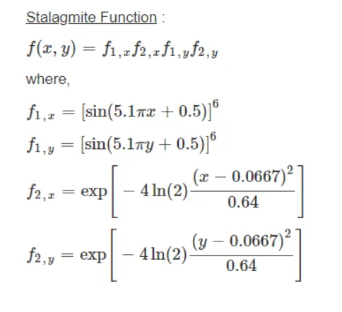
real vectorlb— Lower boundub— Upper boundsnonlcon— Nonlinear constraintsoptions— Optimization optionsIntCon— Integer variableStalagmite Function:-
CODE:-
Stalagmite Function to find Global Minima:-
-
clear all
close all
clc

%Defining our inputs
x = linspace(0,0.6,150);
y = linspace(0,0.6,150);

%Creating 2D mesh
[X Y] = meshgrid(x,y);

% Evaluating stalagmite function
for i=1:length(X)
    for j=1:length(Y)
        input(1) = X(i,j);
        input(2) = Y(i,j);
        f(i,j) = stalagmite(input);   %Calling stalagmite Function
    end
end

surfc(X,Y,f)  % Plotting stalagmite Function
shading interp
[x,fval] = ga(@stalagmite,2) % To find minimum of the function and optimum function value
Stalagmite Function:-
function [f] = stalagmite(input)   % Creating Function

x = input(1);   %Providing inputs
y = input(2);

a1 = (sin(5.1*pi*x + 0.5))^6;
a2 = (sin(5.1*pi*y + 0.5))^6;
a3 = exp(-4*log(2)*((x-0.0667)^2)/0.64);
a4 = exp(-4*log(2)*((y-0.0667)^2)/0.64);

f = a1*a2*a3*a4;
end
Steps:-
- First, we define the inputs array to our code.
- Then we will create a 2D meshing of our Inputs. Then we Assign double loop of out length of our Inputs and defines the stalagmite function inside the loop.
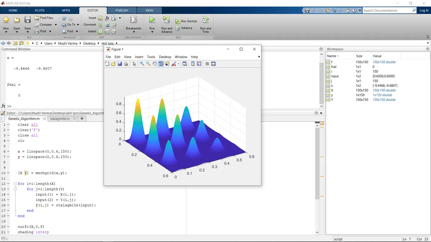
- Then we will use surfc function for 3D plotting of stalagmite function followed by shading interp for creating colored graph.
- Then we will call ga function and inputting stalagmite function into it and then run the code and we get our global minima of stalagmite function.
Result:-
CASE STUDIES FOR GLOBAL MAXIMA:-
CASE-1:- Statistical Behaviour with unbound input:-
clear all
close all
clc

%Defining our inputs
x = linspace(0,0.6,150);
y = linspace(0,0.6,150);
num=50;
%Creating 2D mesh
[X Y] = meshgrid(x,y);

% Evaluating stalagmite function
for i=1:length(X)
    for j=1:length(Y)
        input(1) = X(i,j);
        input(2) = Y(i,j);
        f(i,j) = stalagmite(input);   %Calling stalagmite Function
    end
end

%STUDY-1:- Statistical Behaviour with unbound input

tic
for i=1:num
    [inp,fopt(i)] = ga(@stalagmite,2);
    xopt(i) = inp(1);
    yopt(i) = inp(2);
end
study1_time = toc

figure(1)
subplot(2,1,1)
hold on
surfc(X,Y,-f)
shading interp
xlabel('x-axis')
ylabel('y-axis')
title('Statistical Behaviour with Unbound Inputs')
plot3(xopt,yopt,-fopt,'marker','o','markerSize',4,'markerfacecolor','r')
subplot(2,1,2)
plot(-fopt)
xlabel('Number of Iterations')
ylabel('Maximum points of the function')
Steps:-
- In this we will assign an number=50 to which the number of times the plot will to give an global maxima in unbound conditions
- Then we will run an loop upto length of num to find the optimum points and assign ga function inside the loop.
- Then we plot optimum global maxima point to the stalagmite function plot and also subplot the optimum fuction plot.
Result:-
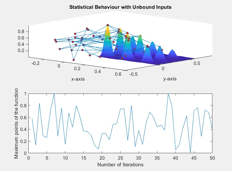
Above, plot show that there are about 350 optimum point from which we can find global maxima in unbound condition.
CASE-2:- Statistical Behaviour with bounded inputs:-
clear all
close all
clc

%Defining our inputs
x = linspace(0,0.6,150);
y = linspace(0,0.6,150);
num=50;
%Creating 2D mesh
[X Y] = meshgrid(x,y);

% Evaluating stalagmite function
for i=1:length(X)
    for j=1:length(Y)
        input(1) = X(i,j);
        input(2) = Y(i,j);
        f(i,j) = stalagmite(input);   %Calling stalagmite Function
    end
end

%STUDY-2:- Statistical Behaviour with upper and lower bound inputs

tic
for i=1:num
    [inp,fopt(i)] = ga(@stalagmite,2,[],[],[],[],[0;0],[0.6;0.6]);
    xopt(i) = inp(1);
    yopt(i) = inp(2);
end
study2_time = toc

figure(2)
subplot(2,1,1)
hold on
surfc(X,Y,-f)
shading interp
xlabel('x-axis')
ylabel('y-axis')
title('Statistical Behaviour with bounded Inputs')
plot3(xopt,yopt,-fopt,'marker','o','markerSize',4,'markerfacecolor','r')
subplot(2,1,2)
plot(-fopt)
xlabel('Number of Iterations')
ylabel('Maximum points of the function')
Steps:-
- In this we will assign an number=50 to which the number of times the plot will to give an global maxima in bounded conditions with upper and lower bound condition.
- Then we will run an loop upto length of num to find the optimum points and assign ga function inside the loop with Aeq and Beq.
- Then we plot optimum global maxima point to the stalagmite function plot and also subplot the optimum fuction plot.
Result:-
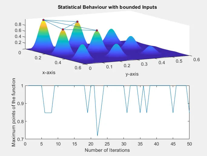
Above, plot show that there are about 4 optimum point from which we can find global maxima in bounded condition. Since this is also not sufficient so we have to increase our statistical cases inside the ga.
CASE-3:- Increasing GA Iterations by increasing population size:-
clear all
close all
clc

%Defining our inputs
x = linspace(0,0.6,150);
y = linspace(0,0.6,150);

%Creating 2D mesh
[X Y] = meshgrid(x,y);

% Evaluating stalagmite function
for i=1:length(X)
    for j=1:length(Y)
        input(1) = X(i,j);
        input(2) = Y(i,j);
        f(i,j) = stalagmite(input);   %Calling stalagmite Function
    end
end

%STUDY-2:- Increasing GA Iterations
options = optimoptions('ga','populationSize',200);
tic
num = 50;
for i=1:num
    [inp,fopt(i)] = ga(@stalagmite,2,[],[],[],[],[0;0],[0.6;0.6],[],[],options);
    xopt(i) = inp(1);
    yopt(i) = inp(2);
end
study4_time = toc

figure(2)
subplot(2,1,1)
hold on
surfc(X,Y,-f)
shading interp
xlabel('x-axis')
ylabel('y-axis')
title('Statistical Behaviour with bounded Inputs with modified population size')
plot3(xopt,yopt,-fopt,'marker','o','markerSize',4,'markerfacecolor','r')
subplot(2,1,2)
plot(-fopt)
xlabel('Number of Iterations')
ylabel('Maximum points of the function')
Steps:-
- In this we will assign an number=50 to which the number of times the plot will to give an global maxima in bounded conditions by increasing the population size upto 200 by using optimoptions function.
- Then we will run an loop upto length of num to find the optimum points and assign ga function inside the loop with Aeq ,Beq and options.
- Then we plot optimum global maxima point to the stalagmite function plot and also subplot the optimum function plot.
Result:-
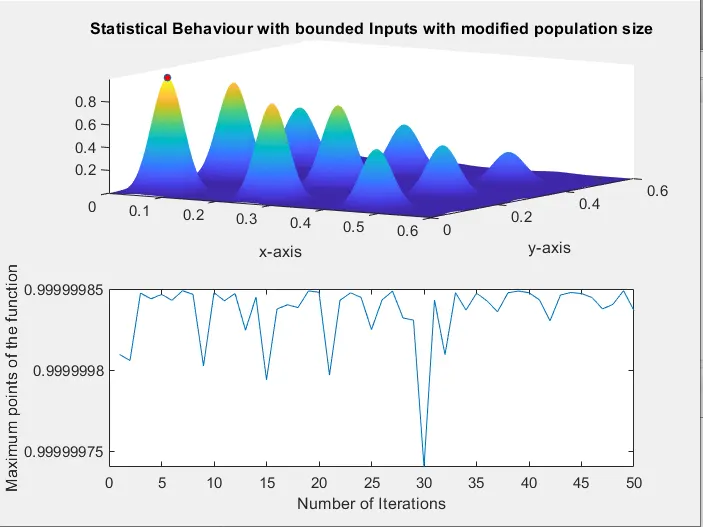
From Above, plot show that there are about 1 optimum point from which we can find global maxima in bounded condition by increasing population size and we get our desired global maxima points.
References:-
https://www.mathworks.com/help/gads/how-the-genetic-algorithm-works.html