Flow over a bicycle

Aim: To calculate the drag force for different velocities and drag coefficients.

Objective : 1) Write a program to plot Velocity vs Drag Force

2) Write a program to plot Drag coefficient vs Drag force

Theory: In fluid dynamics, drag(sometimes called air resistance, a type of friction, or fluid resistance, another type of friction or fluid friction) is a force acting opposite to the relative motion of any object moving with respect to the surrounding fluid).

Drag depends on properties of the fluid and on the size, shape and speed of the object. One way to express this is by means of the drag equation.

Fd = 0.5*rho*v²*Cd*A

Where

Fd is the drag force,

Rho is the density of the fluid

V is the speed of the object relative to the fluid

A is the cross sectional area

Cd is drag coefficient- a dimensionless number

Matlab Code:

% Write a program to plot drag force vs drag coefficient

clear all

close all

clc

% Inputs

% Drag coefficient

c_d = 0.6;

% Frontal area (m^2)

A = 0.1;

% Density (kg/m^2)

Rho = 1.2;

% Velocity

V = (1:50);

Drag_Force = c_d*0.5*Rho*A*V.^2;

figure(1)

plot(V,Drag_Force)

xlabel('Velocity')

ylabel('Dragforce')

grid on

% Program to plot Drag coefficient vs Drag force

V = 10; % Bicycle riding at constant velocity.

c_d = [0.47,0.42,0.50,1.05,0.80,0.82]; % Drag coeffcient for various shapes.

Drag_Force = c_d*0.5*Rho*A*V^2;

figure(2)

plot(c_d,Drag_Force)

xlabel('Drag coefficient')

ylabel('Drag force')

grid on

Explanation of the code:

• The clear all, close all, clc are the commands to clear the workspace as you run the program.
• There are two parts in this program, first part is to write a program to plot velocity vs drag force. Second part is to plot drag coefficient vs drag force.
• Inputs like Drag coefficient, Frontal area, Density are defined. Velocity is defined in matrix of 50 values (1:50).
• Drag force is calculated using the equation. As velocity is a matrix it is multiplied using a dot product.
• The plot of drag force vs velocity is plotted.
• In the second part various values of drag coefficient for different shapes are defined in a matrix. Velocity is kept constant.
• The plot of drag force vs drag coefficient is plotted.

Results:

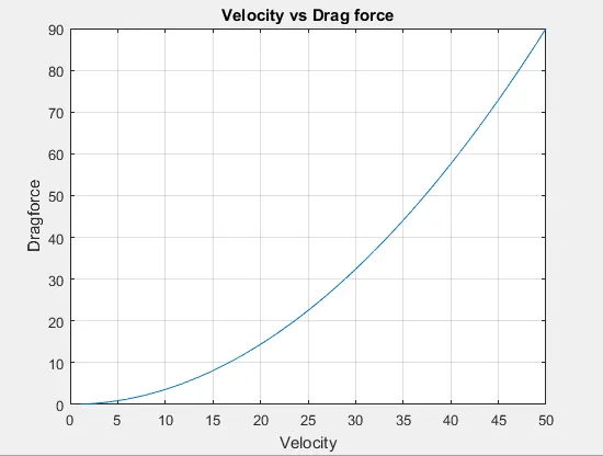
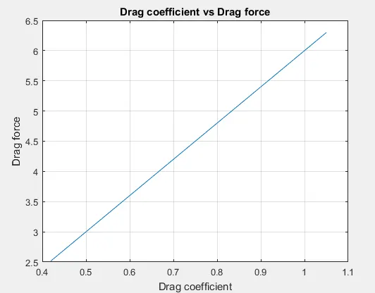
Conclusion: We can see that in the graph of velocity vs drag force, the curve is parabolic as drag force is proportional to the square of the velocity. In the graph of drag coefficient vs drag force, the curve is linear.