Flow over a Backward Facing Step

Introduction

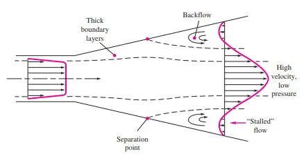
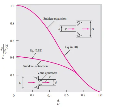
Backward Facing Step is an benchmark model for f low analysis inside a channel with a sudden expansion where friction loss takes place due to the pressure difference. It consists of re-circulation zones(eddies) at the tip of the change in cross-section. The flow reattaches itself at the downstream of the chamber. The re-attachment point is dependent on several factors like inlet fluid velocity, height of the step. If the flow domain is copied and extended on the other side from the axial location in the x direction, it would be a typical expansion flow with certain friction loss. BFS are widely seen in aerodynamic flows (airfoil, spoiler, high attack angle process), engine flows, condensers, vehicles (cars, boat), heat transfer systems, and even the flow around buildings, etc. The flow separation after a simple stage will introduce separation eddies formation, evolution and re-attachment process.

The Backward-Facing Step is also called as “sudden expansion flows”, “back-step flow”, “circular expansion flow” or “diverging channel”. It is an important model for analysis of separation flows with the variationm of Reynolds Number and Drift coefficient.

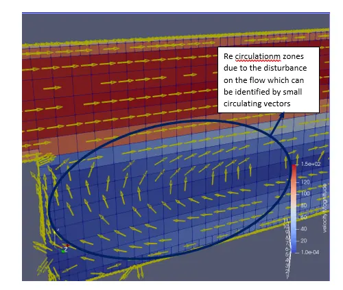
The large separation vortices occur in the backward step region, with a small vortices and secondary vortices in the corner. As instabilities occur, the vortices in the shear layer roll-up and pair with the adjacent vortices to form a coherent structure. The vortices trigger recirculation. Then, due to the presence of an adverse pressure gradient in the wake of the step, the free shear layer reattaches at the bottomstream of the flow domain.

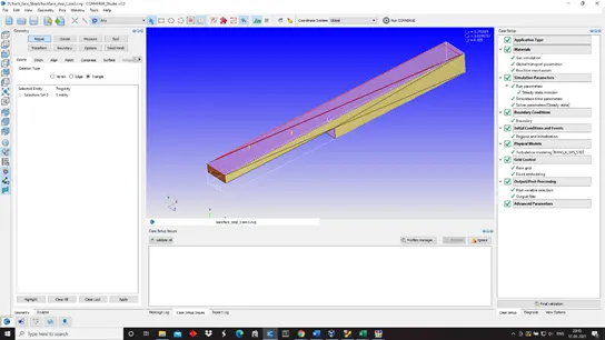
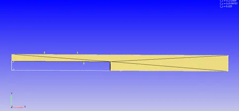
Geometry

CASE SETUP:

Mesh(Grid size)

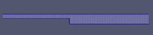
• Case 1~0.002m
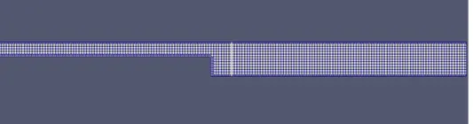
• Case 2~0.0015 m
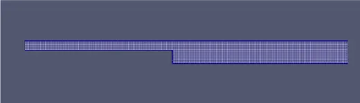
• Case 3~0.001 m

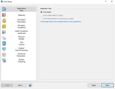
• Time based Setup

• Turbulence Model

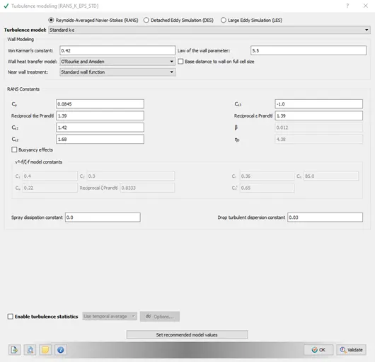
RNG k-€ model is set for this case of steady state analysis.Turbulence Kinetic Energy and Turbulence Dissipation are assigned to default values. The idea revolving turbulencve k-epsilon model is used to normalize ns equations involving Transport Kinmetic Energy(k) and dissipation rate(€) to reduce to the values of k andv €.With these values, Eddy viscosity can be determined from a single turbulent length-scale, so that thr calculated diffuision is that which occurs only at the specified scale. Thev RANS constasnts to be used arev shown as follows.

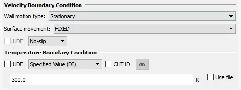
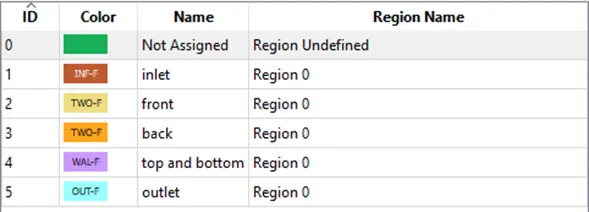
Boundaries

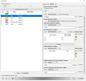
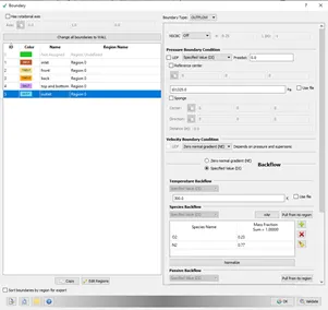
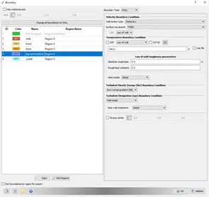
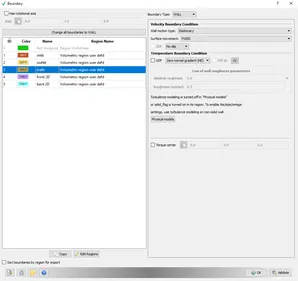
• For materials, air is selected.
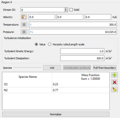
• Initial conditions~ Species-N₂(mass fraction- 0.23and O₂.(mass fraction-0.77) are made to enter the channel domain.

• Run Parameters and Simulation

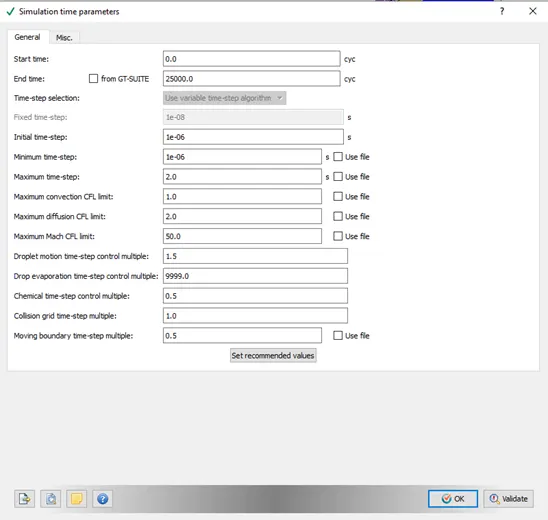
The present hydrodynamic simulation is performed with a steady state solver which non depending on the process path and initial conditions, it will reach steady state and will give somehow tangible results if the geometry and all the other parameters in case-setup is fine. The N-S is set to PISO algorithm which is known to simulate unsteady state problems but also comes in handy with steady states. It uses predictor corrector method in pressure calculation. The simulation is ran for 25000 secs. It is controlled by a steady state solver monitoring at the exit. The steady state monitor starts function at 100 time intervals each and once the avg flow parameter attains steady state the simulation stops.

Time parameters and steady state monitor setup is shown as follows: Total there are 25000 cycles. It is controlled by a steady state solver for the velocityat exit to solve the pressure coupled equation, as said by a predictor-corrector method.The simulation starts functioning at a time interval of 500 cycles and once the avg-velocity attains steady state simulation stops.The average is calculated by taking sample data of specified size( 100 in this case) for which the relative tolerance limit is 0.01.

Pocessing Results in Paraview

• Case 1~0.002m

• Case 2~0.0015 m

• Case 3~0.001 m

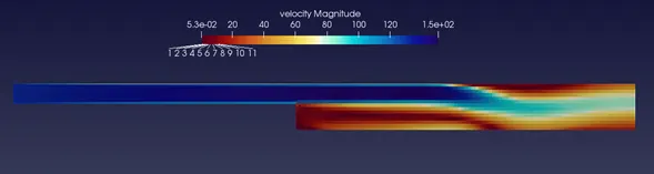
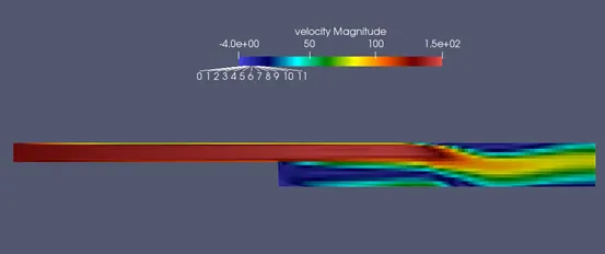
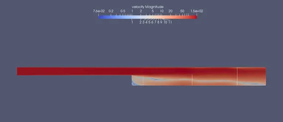
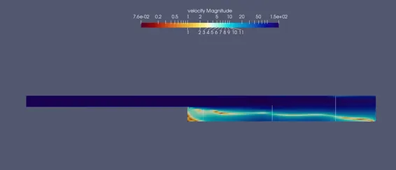
Velocity conmtour

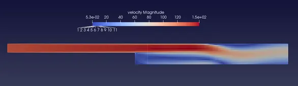
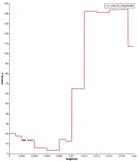
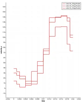
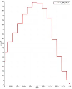
• Case1 : Velocity contour and profile for (a)Case1a:x=0.0136 m;(b)Case 1b:x=0.16,0.19,0.24

(a) (b)

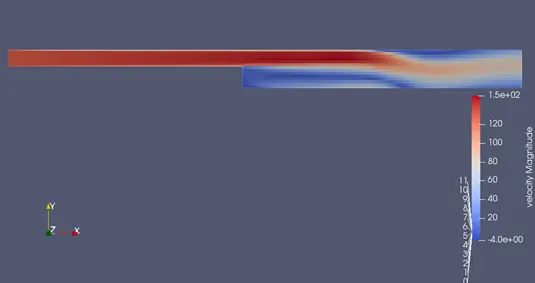
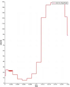
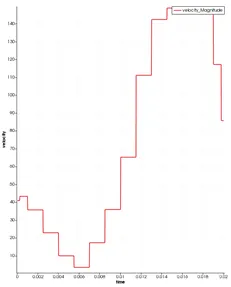
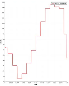
• Case2 : Velocity contour and profile for (a)Case1a:x=0.0136 m;(b)Case 1b:x=0.16(c)Case 1c:x=0.19,(d)Case 1d:x=0.24

(a)

(b)

(c)

(d)

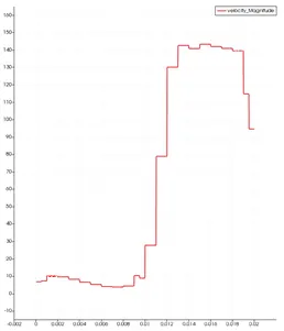
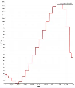
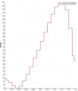
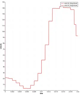
• Case3 : Velocity contour and profile for (a)Case1a:x=0.0136 m;(b)Case 1b:x=0.16(c)Case 1c:x=0.19,(d)Case 1d:X=0.24

(a)

(b)

(c)

(d)

Velocity Vector

Pressure contour

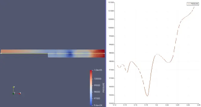
• Case 1

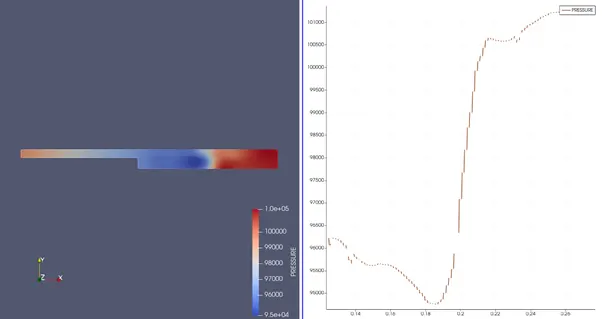
• Case 2

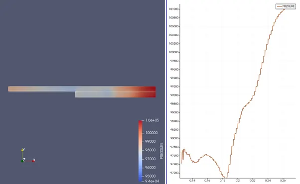
• Case 3

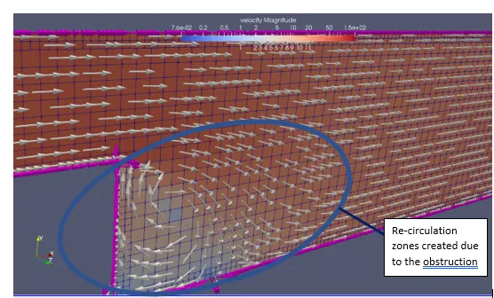
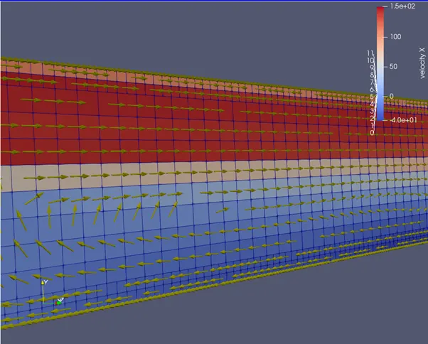
Due to the break(sudden turn in shape causing the obstruction in flow) is causing the fluid to create a recirculate zones which are bettr termed as eddies. In further study it can be shown that with RSM model or DNS or LES simulation how the eddies and the trailing vortex behaves`

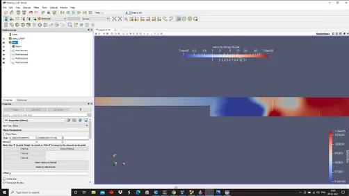
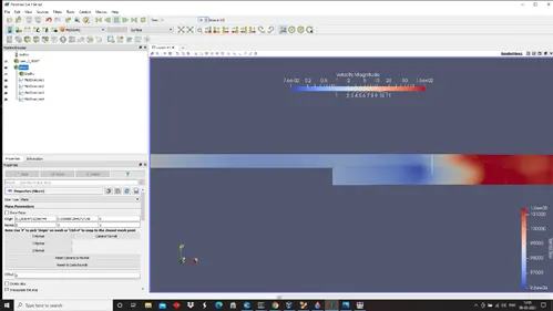
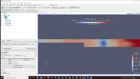
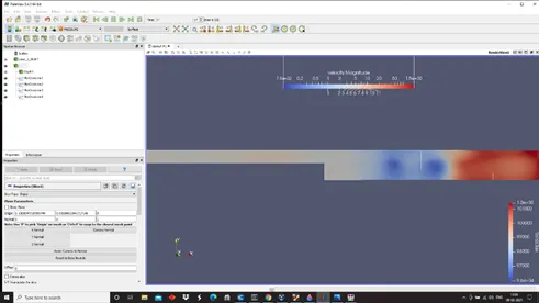
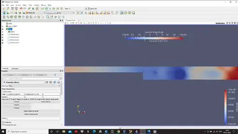
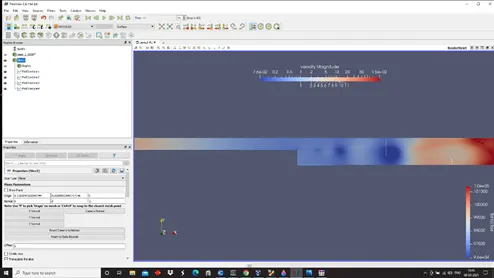
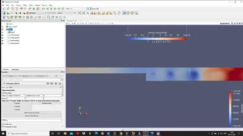
From the below snapshots taken at various flow time for the 3^rd case( flow time~53 s, there is a onset of turbulence near the dam break which is signified by the blue colored low pressure zones. Then the diffusion takes place as the least pressure zone becomes shorter and moves forward with the flow. After that we can see as it moves forward there are trailing vortices which are formed behind the mother vortices which is the least pressure zones. Slowly it gets accumulated at a specific region of low pressure further which the low pressure zone cannot travel which is basically the red colored which has the highest pressure at the exit condition. The Total pressure is 0 at the inlet and the static pressure is 0 at the outlet, and both of them diverges and converges respectively in the regions where they are valid.

• Case 1

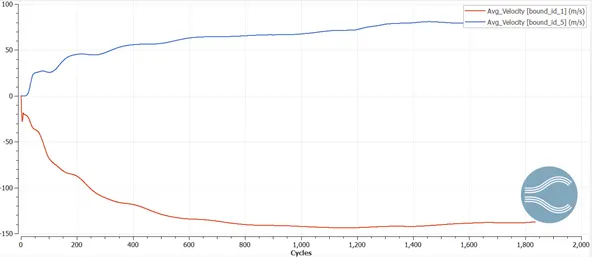
Average Velocity profile (at inklet=-130 m/s; at outlet=52 m/s)

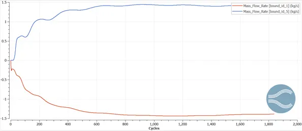
Average Mass Flow Rate( at inlet=-1.4 kg/s; at outlet =1.37 kg/s)

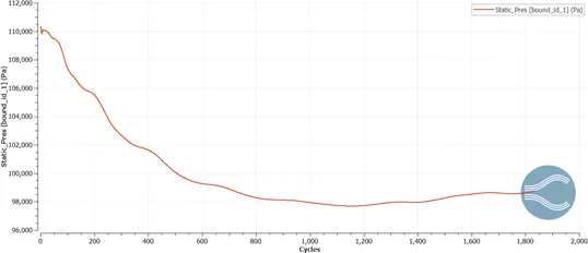
Static Pressure at inlet

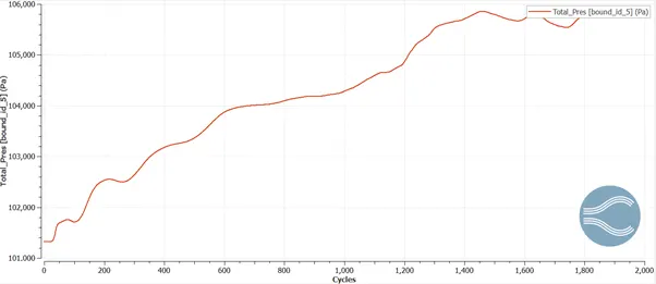
Total Pressure at outlet

• Case 2

Average velocity profile( at inlet=-130 m/s; at outlet=51 m/s)

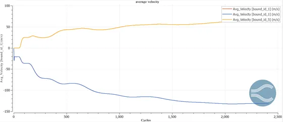
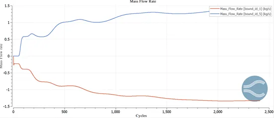
Average Mass Flow Rate (at inlet=-1.3 kg/s; at outlet =1.3 kg/s)

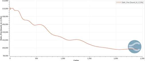
Static Pressure at inlet

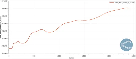
Total Pressure at outlet

• Case 3

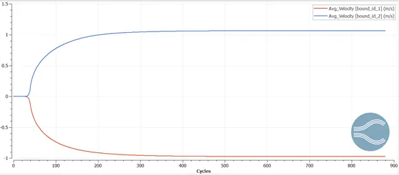
Average velocity profile (at inlet = -1 m/s; at outlet= -1 m/s)

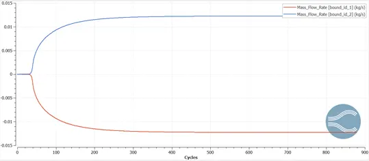
Average Mass Flow Raste( at inlet= -0.025 kg/s; at outlet =0.0156 kg/s)

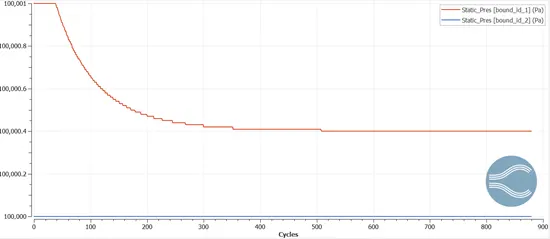
Static Pressure

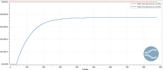
Total Pressure

Conclusions

• As we dec increase the grid size computation time decreases. Damping of the disturbances depends on base the grid size, smaller the base grid size, more cycles are taken to reach a steady state.
• In all the three cases, we can see that the mass flow rate is conserved more or less. The average velocity at the inlet we find is higher than the outlet which must be because of the boundary layer separation or the re-circulation zones created at the sudden expansion region. This is due to the loss of Kinetic Energy in the B.L separation. Static pressure decreases in the re-circulation regions.
• The static pressure is constant at the outlet and decreases at the inlet boundary and the total pressure is constant at the inlet and increases at the outlet. The static pressure is higher at the outlet boundary than the inlet and this is obvious because the height is more than at the inlet. Similarly, the absolute value of total pressure is lesser at the outlet than the inlet where the later is high because of the slight change in pressure from left to right. The total pressure drops at the outlet inferred the direction of flow from left to right.
• The number of cycles that each mesh runs is based on the initial transience of the problem and on the grid size along with the tolerance limit. The initial transience as we can see from the graph settles down when steady state is reached and the simulation stops.

Animations:

• Case 1

• Case 2

• Case 3