Final Project: Electric Rickshaw modelling

Aim:-

To Create a detailed MATLAB model of an Electric Rickshaw (three wheel passenger vehicle).

Objectives:-

• Rear wheels driven by PM brushed type motor
• Assume efficiency points of motor controller and motor
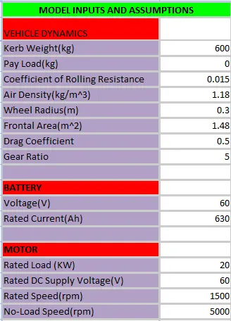
• Make an excel sheet of all input and assumed data 
• Results: For any three standard driving cycles show energy consumption, temperature rise of motor and controller.

Electric Rickshaw:-

Electric rickshaws (also known as electric tuk-tuks or e-rickshaws or toto or e-tricycles) have been becoming more popular in some cities since 2008 as an alternative to auto rickshaws and pulled rickshaws because of their low fuel cost, and less human effort compared to pulled rickshaws. They are being widely accepted as an alternative to petrol/diesel/CNG auto rickshaws. They are three-wheelers powered by an electric motor ranging from 650 to 1400 Watts. They are mostly manufactured in India and China, only a few other countries manufacture these vehicles. Battery-run rickshaws could be a low-emitter complementary transport for the low-income people, who suffer most from a lack of transport facility, if introduced in a systematic manner according to experts.

An auto-rickshaw is a motorized version of the pulled rickshaw or cycle rickshaw. There are many different auto rickshaw designs. The most common type is characterized by a sheet-metal body or open-frame resting on three wheels; a canvas roof with drop-down side curtains; a small cabin at the front for the driver, with handlebar controls; and a cargo, passenger, or dual-purpose space at the rear. Another common type is a motorcycle that has an expanded sidecar or, less often, is pushing or pulling a passenger compartment.

Electric rickshaws have been becoming more popular in some cities since 2008 as an alternative to auto rickshaws and pulled rickshaws because of their low fuel cost, and less human effort compared to pulled rickshaws. They are being widely accepted as an alternative to petrol/diesel/CNG auto-rickshaws. They are three-wheelers powered by an electric motor ranging from 650 to 1400 Watts. They are mostly manufactured in India and China, only a few other countries manufacture these vehicles. Battery-run rickshaws could be a low-emitter complimentary transport for the low-income people, who suffer most from a lack of transport facility if introduced systematically according to experts.

                   

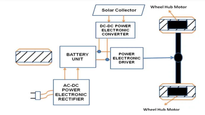
                                                                        Drive train of the Electric Rickshaw

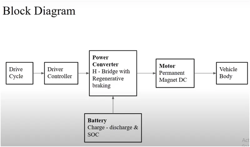
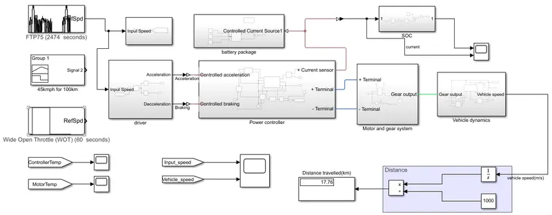
MATLAB modelof Electric Rikshaw:-

Initially the current flows to DC Motor from the battery through the DC-DC power converter to drive the motor. The required voltage will be controlled in the controller. The Controller will follow the given drive cycle reference and run the motor in the required rpm. Then the motor power is transmitted to the wheels of a vehicle through the gear box. and the controller will take the vehicle speed and compare and controlled.

Vehicle Dynamics Sub-system:-

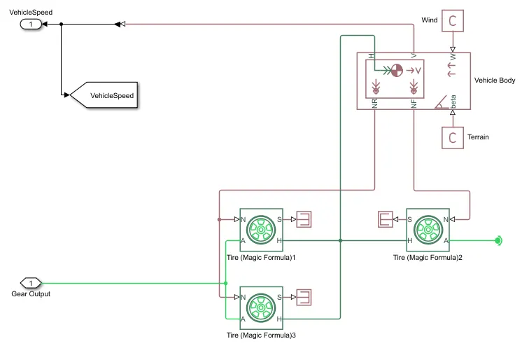
Tire(Magic Formula):-

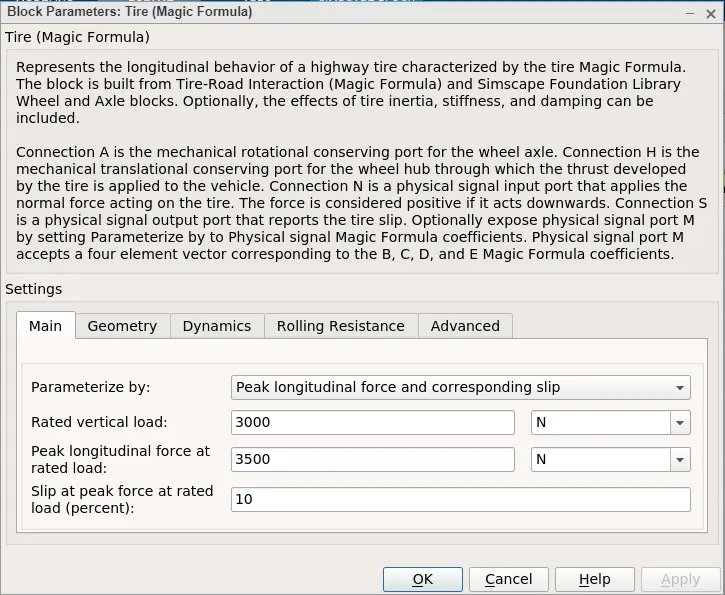
The Tire (Magic Formula) block models a tire with longitudinal behavior given by the Magic Formula , an empirical equation based on four fitting coefficients. The block can model tire dynamics under constant or variable pavement conditions.

The longitudinal direction of the tire is the same as its direction of motion as it rolls on pavement. This block is a structural component based on the Tire-Road Interaction (Magic Formula) block.

To increase the fidelity of the tire model, you can specify properties such as tire compliance, inertia, and rolling resistance. However, these properties increase the complexity of the tire model and can slow down simulation. Consider ignoring tire compliance and inertia if simulating the model in real time or if preparing the model for hardware-in-the-loop (HIL) simulation.

Inputs

N - Normal Force:- Physical signal input port associated with the normal force acting on the tire. The normal force is positive if it acts downward on the tire, pressing it against the pavement.

M - Magic Formula CoPhysical signal input port associated with the Magic Formula coefficients. Provide the Magic Formula coefficients as a four-element vector.

Output

S - Slip :- Physical signal output port associated with the relative slip between the tire and road.

Conserving

A _ Axle:-Mechanical rotational port associated with the axle that the tire sits on.

H - Hub:-Mechanical translational port associated with the wheel hub that transmits the thrust generated by the tire to the remainder of the vehicle.

The tires are parameterized by Peak longitudinal force and corresponding slip.

The other block parameters such as - rated vertical load, peak longitudinal force at rated load and slip at peak force at rated load are kept with their default values.

The tire radius is given as 0.3 m.The tire inertia is kept as 1 kg-m^2.

The rolling resistance is given with a constant coefficient of 0.015.

Vehicle Block:-

The Vehicle Body block represents a two-axle vehicle body in longitudinal motion. The vehicle can have the same or a different number of wheels on each axle. For example, two wheels on the front axle and one wheel on the rear axle. The vehicle wheels are assumed identical in size. The vehicle can also have a center of gravity (CG) that is at or below the plane of travel.

The block accounts for body mass, aerodynamic drag, road incline, and weight distribution between axles due to acceleration and road profile. Optionally include pitch and suspension dynamics. The vehicle does not move vertically relative to the ground.

The block has an option to include an externally-defined mass and an externally-defined inertia. The mass, inertia, and center of gravity of the vehicle body can vary over the course of simulation in response to system changes.

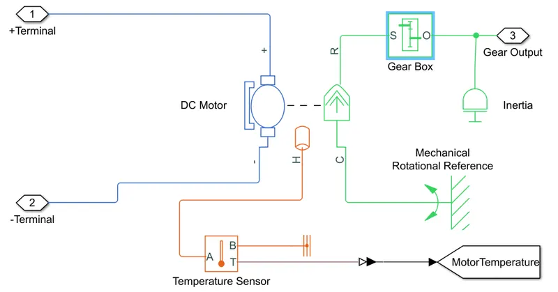
Motor and Gear Sub-System:-

DC Motor:-

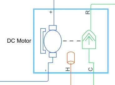
• Simulink provides an inbuilt model block for DC motor which converts electrical input into mechanical rotational output.
• The blue colour corresponds to the electrical side of the motor and the green colour corresponds to the mechanical side .
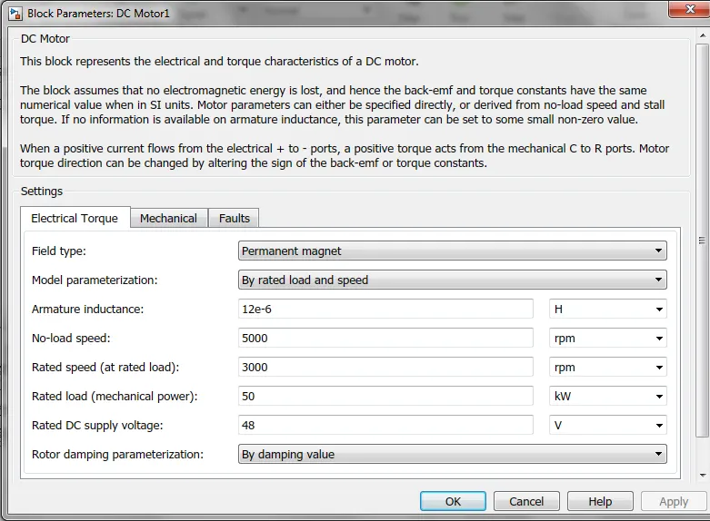
• The motor field type is kept as Permanent magnet and the model parameterization is done by rated load and speed.
• The armature inductance and the mechanical parameters are given their default values.
• The connection R represents the Rotor (rotational output) while the connection C is for the Casing (stationary).
• Thus, the R port is connected to the input of the vehicle subsystem created earlier.
• The C port is connected to a mechanical rotational reference.
• The + and - terminals of the motor are connected to the motor controller.
• If these terminals are directly connected to a battery, the required DC motor will run on the rated capacity of the battery.
• This will eventually result into no control over the DC motor and the vehicle will run at top speed throughout the simulation.

Gear Box:-

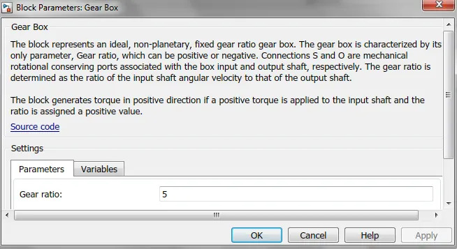
The Gear Box block represents an ideal, nonplanetary, fixed gear ratio gear box. The gear ratio is determined as the ratio of the input shaft angular velocity to that of the output shaft.

The gear box is characterized by its Gear ratio. Here Gear ratio is 5.

Power Controller Sub-System:-

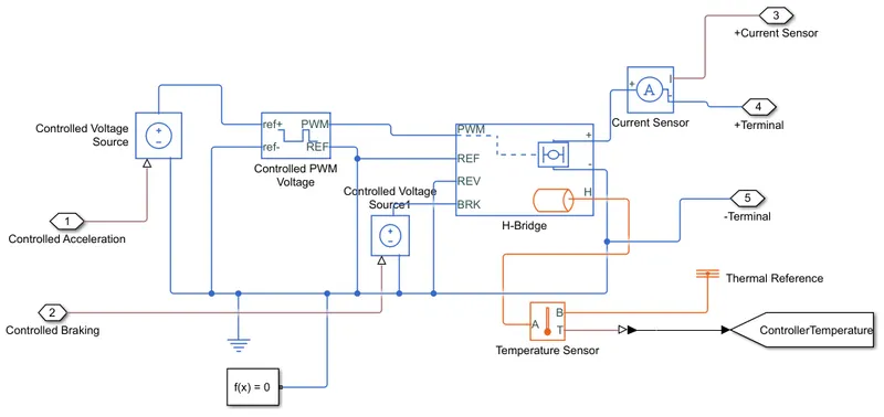
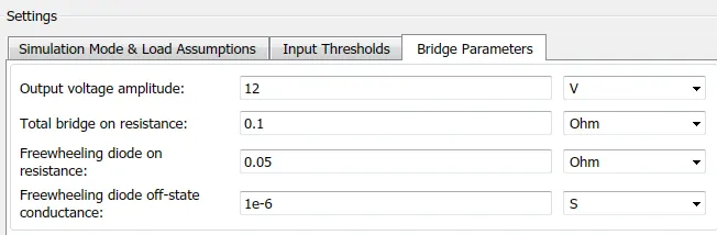
H-Bridge:-

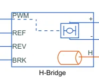
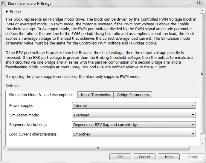
• This block represents an H-bridge motor drive.
• The block can be driven by the Controlled PWM Voltage block in PWM or Averaged mode.
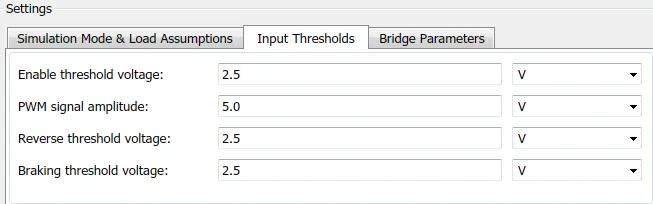
• In PWM mode, the motor is powered if the PWM port voltage is above the enabled threshold voltage.
• In Averaged mode, the PWM port voltage divided by the PWM signal amplitude parameter defines the ratio of the on-time to the PWM period.
• Connection REF is for the reference input.
• This combined with the PWM connected will form the pulse input for the H-Bridge.Here, the REF input is connected to the Electrical Reference (ground).
• Connection REV corresponds to the reverse motion of the motor which essentially means, the backward motion of the vehicle.
• Here, the backward motion of the vehicle is not accounted for and so, the port is connected to the electrical reference.
• Connection BRK is for the braking of the vehicle. Since, the PWM mode results in a huge amount of simulation time, Averaged mode is selected for this simulation.
• Load current characteristics are considered to be smoothed here.
• Also, the regenerative braking is enabled for the simulation. This means, when the vehicle starts decelerating, corresponding amount of charge will be fed back to the battery.
• Accordingly, the BRK input is connected to a Controlled Voltage Source. This will generate emf corresponding to the intensity of brakes applied and fed the power back to the battery.

 

Controlled PVM Voltage:-

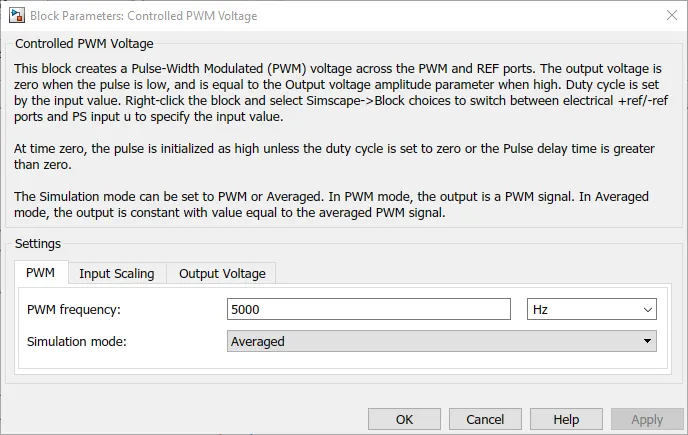
The duty cycle is set by the input value. Right-click the block and select Simscape Block choices to switch between electrical +ref/-ref ports and PS input u to specify the input value. At time zero, the pulse is initialized as high unless the duty cycle is set to zero or the Pulse delay time is greater than zero. The Simulation mode can be set to PWM or Averaged. In PWM mode, the output is a PWM signal. In Averaged mode, the output is constant with a value equal to the averaged PWM signal.

• The PVM port of the Controlled PVM Voltage to the PVM port of the H-Bridge and the REF port to the REF and REV port of the H-bridge.
• Connect the positive port of the Controlled Voltage Source to the ‘ref +’ and the Negative port is connected to the ‘ref –’ along with the electrical reference.
• The physical signal is extended.
• Select all the blocks and create a subsystem named Power Source Unit.

Driver:-

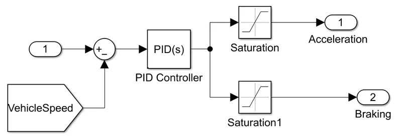
This is the system where the inputs from driver are given the system in terms of speed. To represent the driver input speed, we have used three different blocks i.e. ‘DRIVE CYCLE SOURCE BLOCK’, ‘WIDE OPEN THROTTLE BLOCK’ and ‘SIGNAL BUILDER BLOCK’.

Here we can see that the input speed is fed with feedback of the final vehicle speed and this sum is sent to the ‘PID Controller Block’ so that PID controller will decided whether it has to accelerate or decelerate the vehicle.

Battery Sub-System:-

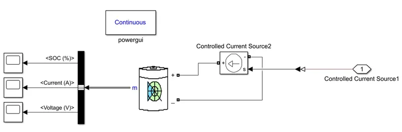
We can see that the current signals from ‘H_BRIDGE’ is connected to this system where first this current signals are converted into physical currents. Using this signals we then have connected it to the ‘BATTERY BLOCK’ where according to these current signal the battery block shows us how much current is used from the battery pack to the match the input current signals, along with this will also show the SOC  and voltage change of the battery.

STATE OF CHARGE:-

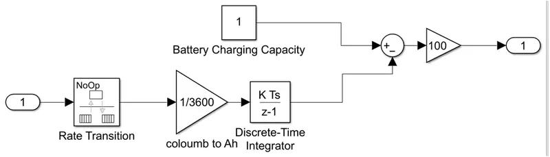
• A small subsystem is created to calculate the State of Charge of the battery.
• This subsystem takes the battery current as the input.
• The essential process to calculate the SOC is by subtracting the charge from the rated capacity of the battery.
• Accordingly, the current is integrated w.r.t. time to get the charge in coulombs.
• Now this coulumb value is modified into Ampere hours. This value is now subtracted from the charging capacity of the battery i.e. 50 Ah.
• Finally, the remaining charge is now converted into percentage value of the charging capacity of the battery

Distance Travelled:-

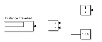
The 2 velocities are first converted from m/s to kmph values. For this, simple Gain blocks are used.The distance is calculated by simply time-integration of the vehicle velocity.

Temperature Sensor:-

Temperature Sensor is used to mesure the temperature of H-Bridge and Motor.

This block measures temperature in a thermal network. There is no heat flow through the sensor. The physical signal port T reports the temperature difference across the sensor. The measurement is positive when the temperature at port A is greater than the temperature at port B.

Solver Configuration:-

Defines solver settings to use for simulation.

References:-

• Electrical Reference: Used to ground the all the electrical connections.
• Mechanical Rotational Reference: Used to ground all the mechanical rotational parts.
• Thermal Reference: Used to ground the thermal sensor.

Results:-

For FTP75 Drive Cycle:-

Run the simulation for 2474sec.

Total Distance Travelled:-

 

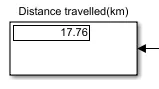
Total distance travelled for FTP75 drive cycle is 17.76km.

Input Speed vs Actual Vehicle Speed:-

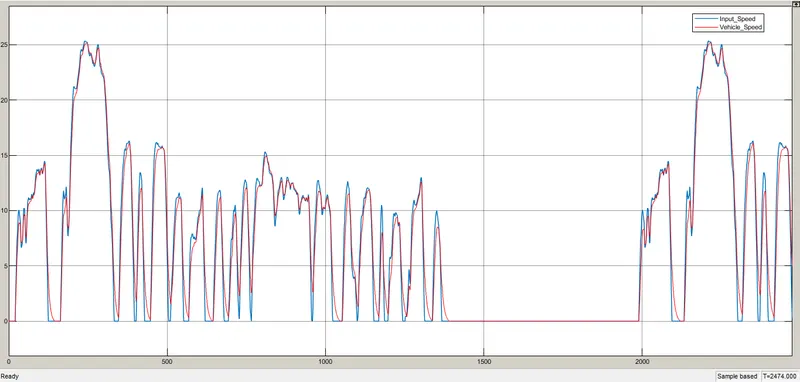
From the above plot, we can observe that vehicle speed is almost similar to the input speed of drive cycle FTP75.

Controller Temperature:-

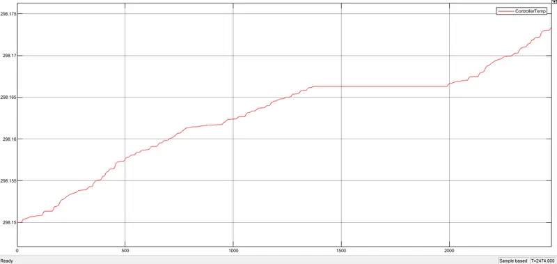
The controller temperature increases slightly from 298.15degrees at starting to 298.175degrees at the completion.

Motor Temperature:-

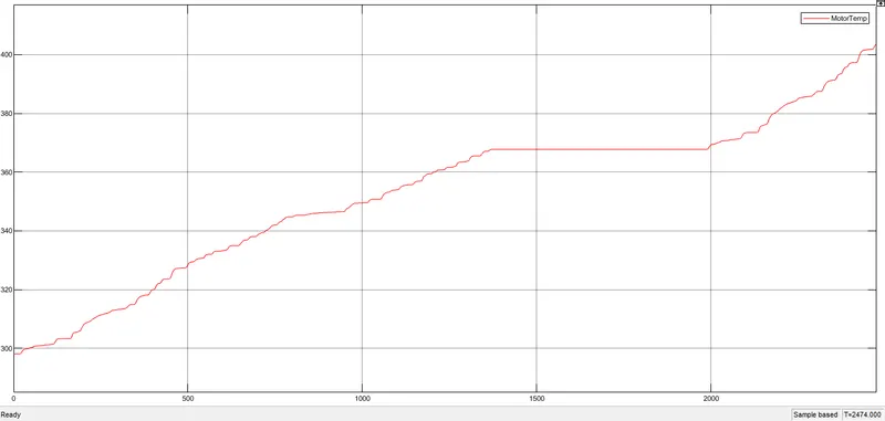
The motor temperature increases from 295degrees at starting to 405degrees at the completion.

SOC and Current:-

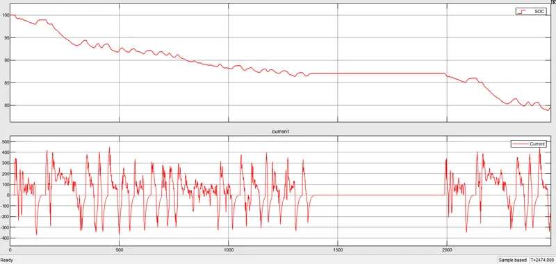
 The charging reduces from 100% to around 80% due to acceleration and regenerative braking.

The current changes as per the speed of the vehicle.

 For 100km with constant speed driving at 45 kmph:-

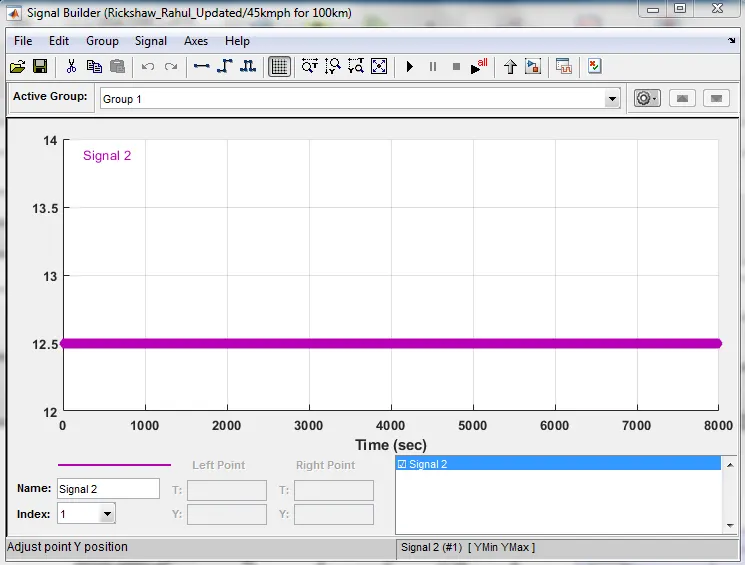
As we have given values in signal builder for 100km distance with constant speed of 45kmph by converting them.

Run the simulation for 8000sec.

  Total Distance Travelled:-

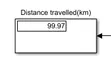
We got the total distance of 99.97km due to the losses.

Input Speed vs Actual Vehicle Speed:-

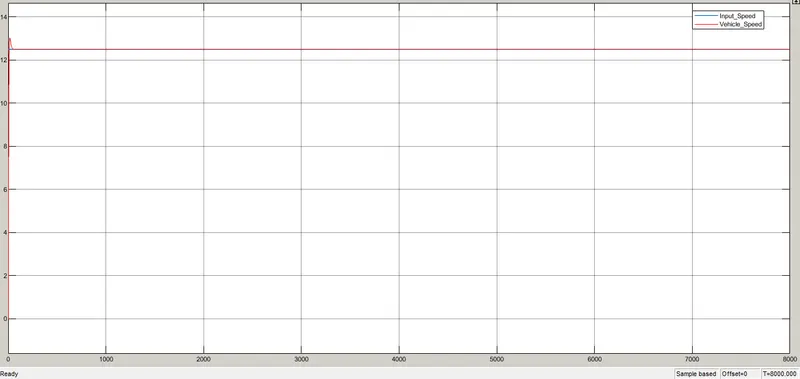
We can observe that, actual speed and input speed colliding with each other at constant speed of 45kmph in entire simulation.

 Controller Temperature:-

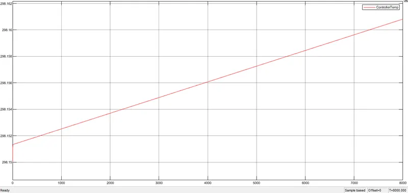
The controller temperature increases very slightly from 298.15degrees at starting to 298.161degrees at the completion as the speed of the vehicle is constant entire simulation.

Motor Temperature:-

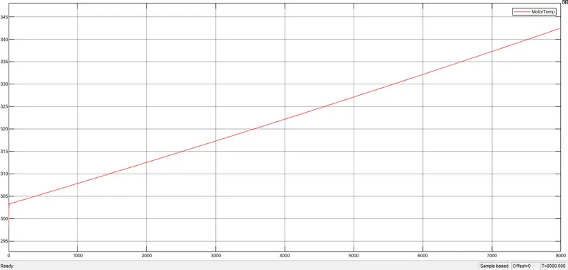
The motor temperature increases  from 300degrees at starting to 342degrees at the completion though the vehicle speed is constant entire simulation and motor is running continuously.

SOC and Current:-

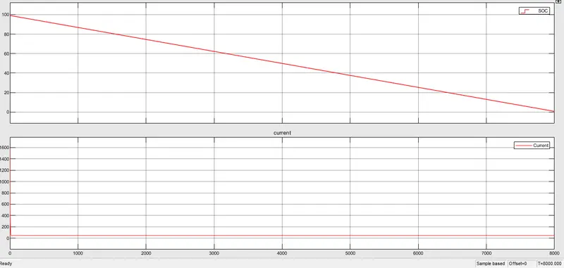
The current value is around 100A and constant through out the simulation as the speed of the vehicle is constant through the simulation.

For WOT (60sec):-

 

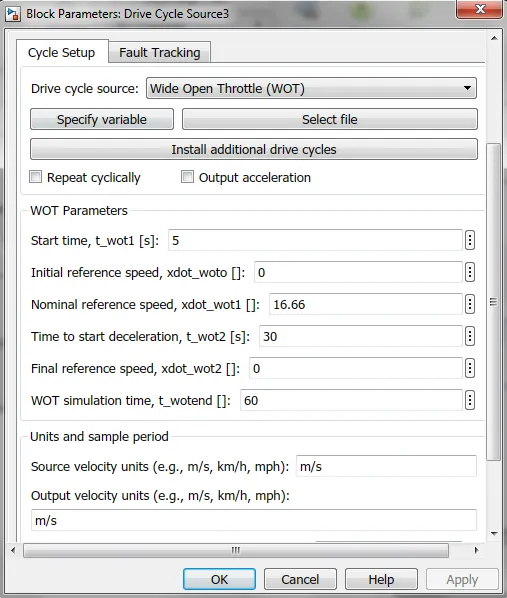
We have given total simulation time for 60sec, WOT start at 5sec and decceleration at 30sec.

Run the simulation for 60sec.

 Total Distance Travelled:-

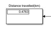
The total distance travelled for 60sec with WOT is 0.4763km.

Input Speed vs Actual Vehicle Speed:-

 

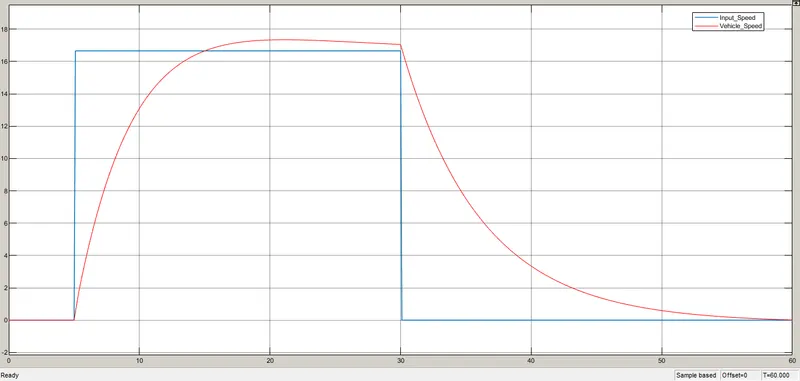
As we can observe that the throttle is opened at 5sec and released at 30sec, which we have given the inputs.

The vehicle speed tried to follow the input and before reaching the specified speed throttle was released from full to zero. The rickshaw could not reach reference speed of 60kmph within 30 seconds

Also, to reach zero after wot is released, it took next 30seconds to reach zero.

SOC and Current:-

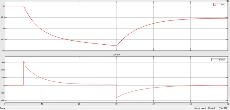
When WOT is opened upto 30sec, the battery charging decreases from 100% to 98.25%

When WOT is released at 30sec, the battery is charged due to regenerative braking from 96.25% to 99.5%

The current increases rapidly from 0 to around 1500A at 5sec as WOT is opened and decreases slowly till the 30th sec and when brake is applied, the current reduces to around-750A and increases to 0 at the end.

Controller Temperature:-

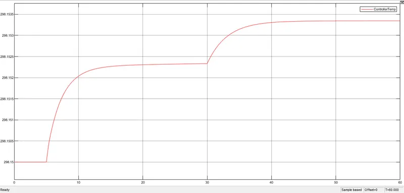
The controller temperature increases very slightly for both WOT period and deceeration period from 298.15degrees to 298.1535degrees.

Motor Temperature:-

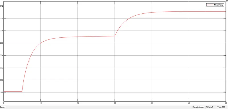
The motor temperature increases  for both WOT period and deceeration period from 298.15degrees to 311degrees as motor is running continuously.