Challenge

Final Project: Electric Rickshaw modelling

KKevin Pinheiro7 Jul 2021

AIM:-To create a MATLAB model of an electric rickshaw with rear wheels driven by PM brushed type motor and to assume efficiency points of motor controller and motor and to make an excel sheet of all input and assumed data.

INTRODUCTION:-

HISTORY:-

Today, the rickshaw represents over a century of rich Indian culture. Originally brought to the country from China, the rickshaw was a hand-pulled vehicle used by traders for transportation of goods. In 1914, the traders asked the governing body for permission to allow the transportation of people as passengers. The request was granted, and rickshaws became a mode of transport for the elite, although now it is used by people of all classes. Since its introduction in 1880, the rickshaw has advanced and evolved into different categories of vehicle: Hand-pulled, cycled, and motorised. Cycle rickshaws began to appear in India around 1930; as the price of bicycles began to fall, the popularity of cycle rickshaws began to rise, and by 1935 the cycle rickshaw outnumbered its hand-pulled counterpart. The auto rickshaw was introduced in 1957 powered by a 250 cc, 8 horsepower, 2 stroke, single-cylinder petrol engine; today, many auto rickshaws are liquified petroleum gas (LPG)
powered. The auto rickshaw’s performance in terms of top speed outclasses both the hand-pulled and cycle rickshaw and is used in a different manner to them. The auto rickshaw is typically used on more open and faster roads, whereas the others are used in narrower and more congested urban environments. It could be argued that the auto rickshaw is not a competitor for the same type of business as the others. All three forms of rickshaw are still in use to this day, compounding their
heritage, tradition, and role within the Indian society. The cycle rickshaw design has not developed a great deal since its introduction and has fallen behind the times in terms of modern-day bicycle design. Bicycles have advanced to a stage where
high-grade lightweight materials and efficient electric motors can make the cyclists ride almost effortless, a vast contrast from the laborious task facing the rickshaw drivers. Cycle rickshaws are heavy and uncomfortable and are therefore exhausting for the drivers to cycle; they are ergonomically inept and often found to be in a poor working condition, only adding to the driver’s exertion.

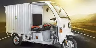
Rickshaw Usage:-
Firstly, regarding the rickshaw performance-wise, it was found that the rickshaw was in use for, on average, 11.36 hours, although not operated during the full 11.36 hours as time would be spent queuing for a passenger. The average daily number of journeys was 28.2, up to a maximum of around 4 km, although a journey of between 1 and 2 km is more typical; therefore, a reasonable approximation of the daily distance could be calculated as 42 km. The rickshaws are fitted with a bench-style seat and are capable of carrying two adults as well as the driver, although 40% of drivers claimed they would carry two adults and a child—this should be disregarded as it was not typical and was only done rarely.

COMPONENTS:-

Motor:-
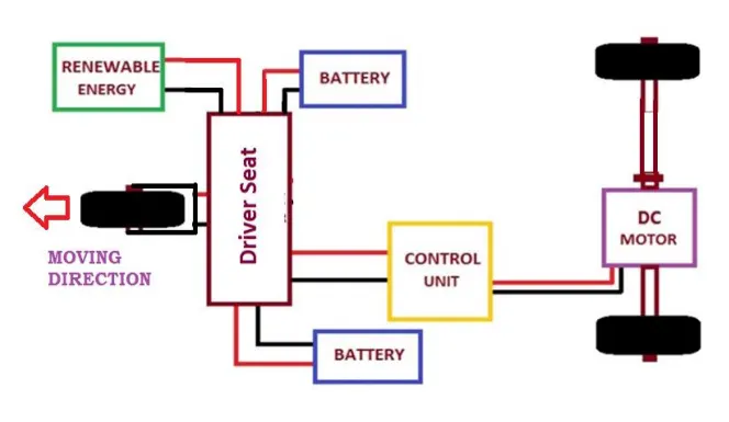
As the results of testing in Section 3.3 showed a highest average of 385.7 W, the motor must be capable of achieving this output. The results were of average wattage; therefore, a larger motor will be needed to meet the peak power demands. The testing was not sufficient to accurately identify peak power as energy expelled, though acceleration up gradient could not be calculated accurately as the increments of gradient were too large; therefore, an estimated simulation was carried out to show a reasonable indication of the peak power. A simulation was executed where it was assumed the driver was accelerating up a slope of 2.06% as per the maximum discovered in testing, assuming they would reach a top speed of 13 km/h in
10 s, though testing this was never achieved, thus being an exaggerated scenario. This will give an overestimation of peak power; therefore, the wattage should be an acceptable measure for a motor that can replicate all human power. The result of the simulation showed a wattage of 468 W; therefore, a 500 W 24 V DC motor is an acceptable choice for the design.

Battery:-
Arguably, the battery is the most important component of an electric vehicle, it has a huge bearing on the range capabilities. There are many considerations that must be satisfied when choosing a battery option such as, cost, ampere hours, voltage, depth of discharge, cycle life, physical size, and weight. From testing in Section 3.3 it was discovered that the motor will require a total of between 2.142 kWh and 2.52 kWh. Taking the higher usage, the Ah capacity can be calculated as 105 Ah.
As stated in the PDS (see Appendix C), the main considerations in the design of the e-rickshaw are cost and range; therefore, the chosen battery must reflect that. Firstly, as cost is the major limitation in this design, the cost of a lithium battery system suitable for the design could cost as much as £1500, based on typical retail prices (March 2019). This consequently rules out the possibility of using lithium batteries in the design. A suitable lead acid battery system would cost around £200 based on typical retail prices (March 2019), which consumes the majority of the budget; therefore, the sourcing of inexpensive refurbished or second-hand units may be the most viable option. Due to the depth of discharge in lead acid batteries being around 50%, achieving a life cycle of 1000 cycles, a system of 4110 Ah units will be installed in a circuit of 2 parallel branches; this will provide the motor with the 24 V needed and a capacity of 210 Ah, assuming a depth of discharge
(DOD) of 50% a usable capacity of 110 Ah, which exceeds the targeted range.

Gearing:-
Commonly in India, the rickshaws are fitted with a singular gear and therefore unable to change torque for different gradients and speeds; this is largely due to cost reduction, lower maintenance, and for simplicity of design. This fits with the PDS brief and therefore should be continued. The pedal sprocket transfers the human power onto the rear shaft via a link chain and a gear attached to the shaft, and the power can be stepped up or stepped down by a multitude of gear sizes. Typically, on a rickshaw the ratio is 1:0.56 and the pedal sprocket of 48 teeth is stepped down to a 27 tooth on the rear shaft therefore, for every one full pedal cycle, the rear shaft rotates 1.778 times; the rickshaw, neglecting any losses in grips at the wheels, should move 1.778 times the circumference of the rear wheels. With this ratio, a pedal sprocket cadence of 90 RPM would propel the rickshaw at a speed of 20 km/h, and this is acceptable for the final design; although, this ratio does not suit acceleration, and therefore must be replaced with a ratio that reduces the physical efforts of the driver. A ratio of 1:1
will provide the driver with increased torque allowing the easier rotation of the pedals and will drive at a speed of 11 km/h at a cadence of 90 RPM. It is important to keep the gearing ratio to a reasonably achievable speed; if an electric component fails, then the driver may still be able to cycle manually and either complete his shift or take the rickshaw to a repair centre.
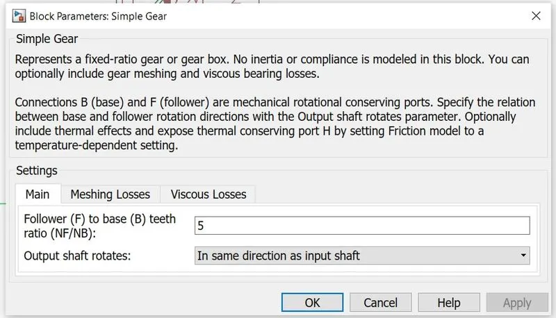
The gearing of the motor will be set to provide the vehicle with a top speed of 15 km/h; since the rated RPM of the motor is 2500, the gearing must step the RPM down to 192, using a gear ratio 1:13 this. In theory, can be achieved.

BLOCKS USED:-

DRIVE CYCLE SOURCE:-

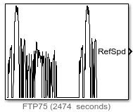
The Drive Cycle Source block generates a standard or user-specified longitudinal drive cycle. The block output is the specified vehicle longitudinal speed, which you can use to:

Predict the engine torque and fuel consumption that a vehicle requires to achieve desired speed and acceleration for a given gear shift reference.
Produce realistic velocity and shift references for closed loop acceleration and braking commands for vehicle control and plant models.
Study, tune, and optimize vehicle control, system performance, and system robustness over multiple drive cycles.
Identify the faults within tolerances specified by standardized tests, including:
- EPA dynamometer driving schedules¹
- Worldwide Harmonised Light Vehicle Test Procedure (WLTP) laboratory tests²

SCOPE:-

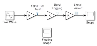
Simulink^® scopes provide several methods for displaying simulation data and capturing the data for later analysis. Symbols on your block diagram represent the various data display and data capture methods.

LONGITUDINAL DRIVER BLOCK:-

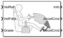
The Longitudinal Driver block implements a longitudinal speed-tracking controller. Based on reference and feedback velocities, the block generates normalized acceleration and braking commands that can vary from 0 through 1. You can use the block to model the dynamic response of a driver or to generate the commands necessary to track a longitudinal drive cycle.

CONTROLLED VOLTAGE SOURCE:-

The Controlled Voltage Source block represents an ideal voltage source that is powerful enough to maintain the specified voltage at its output regardless of the current flowing through the source.

The output voltage is V = Vs, where Vs is the numerical value presented at the physical signal port.

CONTROLLED PWM VOLTAGE:-

The Controlled PWM Voltage block represents a pulse-width modulated (PWM) voltage source. The block has two modeling variants, accessible by right-clicking the block in your block diagram and then selecting the appropriate option from the context menu, under Simscape > Block choices:

Electrical input ports — The block calculates the duty cycle based on the reference voltage across its ref+ and ref- ports. This modeling variant is the default.
PS input — Specify the duty cycle value directly by using an input physical signal port.

For the Electrical input ports variant of the block, the demanded duty cycle is

100∗Vref−VminVmax−Vmin percent

where:

V_ref is the reference voltage across the ref+ and ref- ports.
V_min is the minimum reference voltage.
V_max is the maximum reference voltage.

H-BRIDGE:-

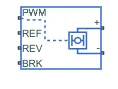
The H-Bridge block represents an H-bridge motor driver. The block has the following two Simulation mode options:

PWM — The H-Bridge block output is a controlled voltage that depends on the input signal at the PWM port. If the input signal has a value greater than the Enable threshold voltage parameter value, the H-Bridge block output is on and has a value equal to the value of the Output voltage amplitude parameter. If it has a value less than the Enable threshold voltage parameter value, the block maintains the load circuit using one of the following three Freewheeling mode options:
- Via one semiconductor switch and one freewheeling diode
- Via two freewheeling diodes
- Via two semiconductor switches and one freewheeling diode
The first and third options are sometimes referred to as synchronous operation.

The signal at the REV port determines the polarity of the output. If the value of the signal at the REV port is less than the value of the Reverse threshold voltage parameter, the output has positive polarity; otherwise, it has negative polarity.
Averaged — This mode has two Load current characteristics options:
- Smoothed
- Unsmoothed or discontinuous
The Smoothed option assumes that the current is practically continuous due to load inductance. In this case, the H-Bridge block output is:

VOVPWMAPWM−IOUTRON

where:
- V_O is the value of the Output voltage amplitude parameter.
- V_PWM is the value of the voltage at the PWM port.
- A_PWM is the value of the PWM signal amplitude parameter.
- I_OUT is the value of the output current.
- R_ON is the Bridge on resistance parameter.
The current will be smooth if the PWM frequency is large enough. Synchronous operation where freewheeling is via a bridge arm back to the supply also helps smooth the current. For cases where the current is not smooth, or possibly discontinuous (that is, it goes to zero between PWM cycles), use the Unsmoothed or discontinuous option. For this option, you must also provide values for the Total load series resistance, Total load series inductance, and PWM frequency. During simulation, the block uses these values to calculate a more accurate value for H-bridge output voltage that achieves the same average current as would be present if simulating in PWM mode.

Set the Simulation mode parameter to Averaged to speed up simulations when driving the H-Bridge block with a Controlled PWM Voltage block. You must also set the Simulation mode parameter of the Controlled PWM Voltage block to Averaged mode. This applies the average of the demanded PWM voltage to the motor. The accuracy of the Averaged mode simulation results relies on the validity of your assumption about the load current. If you specify that the current is Unsmoothed or discontinuous, then the accuracy also depends on the values you provide for load resistance and inductance being representative. This mode also makes some simplifying assumptions about the underlying equations for the case when current is discontinuous. For typical motor and bridge parameters, accuracy should be within a few percent. To verify Averaged mode accuracy, run the simulation using the PWM mode and compare the results to those obtained from using the Averaged mode.

Braking mode is invoked when the voltage presented at the BRK port is larger than the Braking threshold voltage. Regardless of whether in PWM or Averaged mode, when in braking mode the H-bridge is modeled by a series combination of two resistances R1 and R2 where:

R1 is the resistance of a single bridge arm, that is, half the value of the Total bridge on resistance parameter.
R2 is the resistance of a single bridge arm in parallel with a diode resistance, that is, R1 · Rd / ( R1 + Rd ), where Rd is the diode resistance.

CURRENT SENSOR:-

The Current Sensor block represents an ideal current sensor, that is, a device that converts current measured in any electrical branch into a physical signal proportional to the current.

Connections + and – are electrical conserving ports through which the sensor is inserted into the circuit. Connection I is a physical signal port that outputs the measurement result.

VOLTAGE SENSOR:-

The Voltage Sensor block represents an ideal voltage sensor, that is, a device that converts voltage measured between two points of an electrical circuit into a physical signal proportional to the voltage.

Connections + and – are electrical conserving ports through which the sensor is connected to the circuit. Connection V is a physical signal port that outputs the measurement result.

DC MOTOR:-

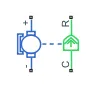
The DC Motor block represents the electrical and torque characteristics of a DC motor using the following equivalent circuit model:

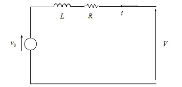
You specify the equivalent circuit parameters for this model when you set the Model parameterization parameter to By equivalent circuit parameters. The resistor R corresponds to the resistance you specify in the Armature resistance parameter. The inductor L corresponds to the inductance you specify in the Armature inductance parameter.

You can specify how to generate the magnetic field of the DC motor by setting the Field type parameter to the desired option. The permanent magnets in the motor induce the following back emf v_b in the armature:

vb=kvω

where k_v is the Back-emf constant and ω is the angular velocity. The motor produces the following torque, which is proportional to the motor current i:

TE=kti

where k_t is the Torque constant. The DC Motor block assumes that there are no electromagnetic losses. This means that mechanical power is equal to the electrical power dissipated by the back emf in the armature. Equating these two terms gives:

TEω=vbiktiω=kvωikv=kt

As a result, you specify either k_v or k_t in the block parameters.

If the magnetic field is generated from the current flowing through the windings, the Back-emf constant depends on the field current I_f:

kv=LafIf

where L_af is the Field-armature mutual inductance.

The torque-speed characteristic for the DC Motor block is related to the parameters in the preceding figure. When you set the Model parameterization parameter to By stall torque & no-load speed or By rated power, rated speed & no-load speed, the block solves for the equivalent circuit parameters as follows:

For the steady-state torque-speed relationship, L has no effect.
Sum the voltages around the loop and rearrange for i:

i=V−vbR=V−kvωR
Substitute this value of i into the equation for torque:

TE=ktR(V−kvω)

When you set the Model parameterization parameter to By stall torque & no-load speed, the block uses the preceding equation to determine values for R and k_t (and equivalently k_v).

When you set the Model parameterization parameter to By rated power, rated speed & no-load speed, the block uses the rated speed and power to calculate the rated torque. The block uses the rated torque and no-load speed values in the preceding equation to determine values for R and k_t.

The block models motor inertia J and damping λ for all values of the Model parameterization parameter. The resulting torque across the block is:

T=ktR(V−kvω)−J˙ω−λω

It is not always possible to measure rotor damping, and rotor damping is not always provided on a manufacturer datasheet. An alternative is to use the no-load current to infer a value for rotor damping.

For no-load, the electrically-generated mechanical torque must equal the rotor damping torque:

ktinoload=λωnoload

where i_noload is the no-load current. If you select By no-load current for the Rotor damping parameterization parameter, then this equation is used in addition to the torque-speed equation to determine values for λ and the other equation coefficients.

The value for rotor damping, whether specified directly or in terms of no-load current, is taken into account when determining equivalent circuit parameters for Model parameterization options By stall torque and no-load speed and By rated power, rated speed and no-load speed.

When a positive current flows from the electrical + to - ports, a positive torque acts from the mechanical C to R ports.

Faults

The DC Motor block allows you to model two types of faults:

Armature winding fault — The armature winding fails and goes open circuit.
Field winding fault — The field winding that creates the magnetic field fails and goes open circuit.

The block can trigger fault events:

At a specific time (temporal fault).
When a current limit is exceeded for longer than a specific time interval (behavioral fault).

You can enable or disable these trigger mechanisms separately.

You can choose whether to issue an assertion when a fault occurs, by using the Reporting when a fault occurs parameter. The assertion can take the form of a warning or an error. By default, the block does not issue an assertion.

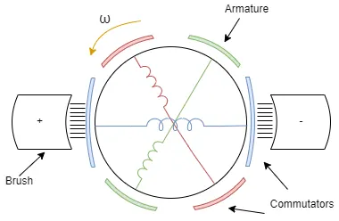
This figure shows a generic representation of a DC motor, with brushes, armatures, commutators, and their windings:

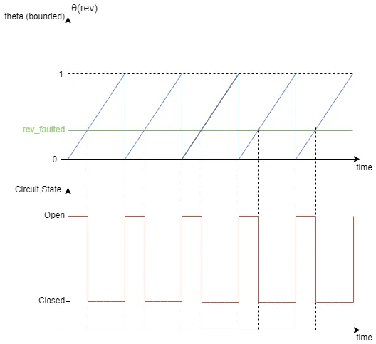
If you set the Enable armature winding open-circuit fault parameter to Yes, the armature fails at the time specified by the Time at which armature winding fault is triggered parameter for a temporal fault, or when the winding currents exceeds the value of the Maximum permissible armature winding current parameter for a behavioral fault. When the armature fails, the voltage source connected to this block observes an open circuit for a fraction of the total motor revolution, specified by the Fraction of revolution during which armature is open-circuit parameter, rev_faulted. This figure illustrates the circuit state behaviour for a certain rev_faulted during the entire revolution period:

Thermal Port

The block has an optional thermal port, hidden by default. To expose the thermal port, right-click the block in your model, and then from the context menu select Simscape > Block choices > Show thermal port. This action displays the thermal port H on the block icon, and exposes the Temperature Dependence and Thermal Port parameters.

Use the thermal port to simulate the effects of copper resistance losses that convert electrical power to heat. For more information on using thermal ports and on the Temperature Dependence and Thermal Port parameters.

TEMPERATURE SENSOR:-

The Temperature Sensor block represents an ideal temperature sensor, that is, a device that determines the temperature differential measured between two points without drawing any heat.

Connections A and B are thermal conserving ports that connect to the two points where temperature is being monitored. Port T is a physical signal port that outputs the temperature differential value.

The block positive direction is from port A to port B. The measured temperature is determined as T = T_A – T_B.

CONSTANT:-

The Constant block generates a real or complex constant value signal. Use this block to provide a constant signal input. The block generates scalar, vector, or matrix output, depending on:

The dimensionality of the Constant value parameter
The setting of the Interpret vector parameters as 1-D parameter

The output of the block has the same dimensions and elements as the Constant value parameter. If you specify for this parameter a vector that you want the block to interpret as a vector, select the Interpret vector parameters as 1-D check box. Otherwise, if you specify a vector for the Constant value parameter, the block treats that vector as a matrix.

PRODUCT:-

The Product block outputs the result of multiplying two inputs: two scalars, a scalar and a nonscalar, or two nonscalars that have the same dimensions. The default parameter values that specify this behavior are:

Multiplication: Element-wise(.*)
Number of inputs: 2

INTEGRATOR:-

The Integrator block outputs the value of the integral of its input signal with respect to time.

Simulink^® treats the Integrator block as a dynamic system with one state. The block dynamics are given by:

{˙x(t)y(t)=u(t)=x(t) x(t0)=x0

where:

u is the block input.
y is the block output.
x is the block state.
x₀ is the initial condition of x.

While these equations define an exact relationship in continuous time, Simulink uses numerical approximation methods to evaluate them with finite precision. Simulink can use several different numerical integration methods to compute the output of the block, each with advantages in particular applications. Use the Solver pane of the Configuration Parameters dialog box (see Solver Pane) to select the technique best suited to your application.

The selected solver computes the output of the Integrator block at the current time step, using the current input value and the value of the state at the previous time step. To support this computational model, the Integrator block saves its output at the current time step for use by the solver to compute its output at the next time step. The block also provides the solver with an initial condition for use in computing the block's initial state at the beginning of a simulation. The default value of the initial condition is 0. Use the block parameter dialog box to specify another value for the initial condition or create an initial value input port on the block.

Use the parameter dialog box to:

Define upper and lower limits on the integral
Create an input that resets the block's output (state) to its initial value, depending on how the input changes
Create an optional state output so that the value of the block's output can trigger a block reset

Use the Discrete-Time Integrator block to create a purely discrete system.

Defining Initial Conditions

You can define the initial conditions as a parameter on the block dialog box or input them from an external signal:

To define the initial conditions as a block parameter, specify the Initial condition source parameter as internal and enter the value in the Initial condition field.
To provide the initial conditions from an external source, specify the Initial condition source parameter as external. An additional input port appears under the block input.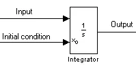

Limiting the Integral

To prevent the output from exceeding specifiable levels, select the Limit output check box and enter the limits in the appropriate parameter fields. This action causes the block to function as a limited integrator. When the output reaches the limits, the integral action is turned off to prevent integral wind up. During a simulation, you can change the limits but you cannot change whether the output is limited. The block determines output as follows:

When the integral is less than or equal to the Lower saturation limit, the output is held at the Lower saturation limit.
When the integral is between the Lower saturation limit and the Upper saturation limit, the output is the integral.
When the integral is greater than or equal to the Upper saturation limit, the output is held at the Upper saturation limit.

To generate a signal that indicates when the state is being limited, select the Show saturation port check box. A saturation port appears below the block output port.

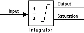
The signal has one of three values:

1 indicates that the upper limit is being applied.
0 indicates that the integral is not limited.
–1 indicates that the lower limit is being applied.

When you select this check box, the block has three zero crossings: one to detect when it enters the upper saturation limit, one to detect when it enters the lower saturation limit, and one to detect when it leaves saturation.

Wrapping Cyclic States

Several physical phenomena are cyclic, periodic, or rotary in nature. Objects or machinery that exhibit rotational movement and oscillators are examples of such phenomena.

Modeling these phenomena in Simulink involves integrating the rate of change of the periodic or cyclic signals to obtain the state of the movement.

The drawback with this approach, however, is that over long simulation time spans, the states representing periodic or cyclic signals integrate to large values. Further, computing the sine or cosine of these signals takes an increasingly large amount of time because of angle reduction. The large signals values also negatively impact solver performance and accuracy.

One approach for overcoming this drawback is to reset the angular state to 0 when it reaches 2π (or to –π when it reaches π, for numerical symmetry). This approach improves the accuracy of sine and cosine computations and reduces angle reduction time. But it also requires zero-crossing detection and introduces solver resets, which slow down the simulation for variable step solvers, particularly in large models.

To eliminate solver resets at wrap points, the Integrator block supports wrapped states that you can enable by checking Wrap state on the block parameter dialog box. When you enable Wrap state, the block icon changes to indicate that the block has wrapping states.

Simulink allows wrapping states that are bounded by upper and lower values parameters of the wrapped state. The algorithm for determining wrapping states is given by:

y=xx−(xu−xl)Ax−xlxu−xlBx∈[xl,xu)otherwise

where:

x_l is the lower value of the wrapped state.
x_u is the upper value of the wrapped state.
y is the output.

The support for wrapping states provides these advantages.

It eliminates simulation instability when your model approaches large angles and large state values.
It reduces the number of solver resets during simulation and eliminates the need for zero-crossing detection, improving simulation time.
It eliminates large angle values, speeding up computation of trigonometric functions on angular states.
It improves solver accuracy and performance and enables unlimited simulation time.

Resetting the State

The block can reset its state to the specified initial condition based on an external signal. To cause the block to reset its state, select one of the External reset choices. A trigger port appears below the block's input port and indicates the trigger type.

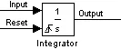
Select rising to reset the state when the reset signal rises from a negative or zero value to a positive value.
Select falling to reset the state when the reset signal falls from a positive value to a zero or negative value.
Select either to reset the state when the reset signal changes from zero to a nonzero value, from a nonzero value to zero, or changes sign.
Select level to reset the state when the reset signal is nonzero at the current time step or changes from nonzero at the previous time step to zero at the current time step.
Select level hold to reset the state when the reset signal is nonzero at the current time step.

The reset port has direct feedthrough. If the block output feeds back into this port, either directly or through a series of blocks with direct feedthrough, an algebraic loop results (see Algebraic Loop Concepts). Use the Integrator block's state port to feed back the block's output without creating an algebraic loop.

POWER GUI:-

Description

The powergui block allows you to choose one of these methods to solve your circuit:

Continuous, which uses a variable-step solver from Simulink^®
Discretization of the electrical system for a solution at fixed time steps
Continuous or discrete phasor solution

The powergui block also opens tools for steady-state and simulation results analysis and for advanced parameter design.

You need the powergui block to simulate any Simulink model containing Simscape™ Electrical™ Specialized Power Systems blocks. It stores the equivalent Simulink circuit that represents the state-space equations of the model.

When using one powergui block in a model:

Place the powergui block in the top-level diagram for optimal performance.
Make sure that the block is named powergui.

CONTROLLED CURRENT SOURCE:-

The Controlled Current Source block converts the Simulink^® input signal into an equivalent current source. The generated current is driven by the input signal of the block. The positive current direction is as shown by the arrow in the block icon.

You can initialize the Controlled Current Source block with a specific AC or DC current. If you want to start the simulation in steady state, the block input must be connected to a signal starting as a sinusoidal or DC waveform corresponding to the initial values.

Parameters

Initialize

Default is selected. If selected, initializes the Controlled Current Source block with the specified Initial current, Initial phase, and Initial frequency parameters.

Source type

The Source type parameter is not visible if the Initialize parameter is not selected.

The type of current source. Select AC (default) to initialize the Controlled Current Source Block as an AC current source. Select DC to initialize the Controlled Current Source block as a DC current.

Initial amplitude

This parameter is not visible in the dialog box if the Initialize parameter is cleared. The initial peak current for the initialization of the source, in amperes (A). Default is 0.

Initial phase

The initial phase for the initialization of the source, in degrees. Default is 0. The Initial phase parameter is not visible in the dialog box if the Source type parameter is set to DC.

Initial frequency

The initial frequency for the initialization of the source, in hertz (Hz). Default is 0. The Initial frequency parameter is not visible in the dialog box if the Source type parameter is set to DC.

Measurements

Default is None. Select Current to measure the current flowing through the Controlled Current Source block.

BATTERY:-

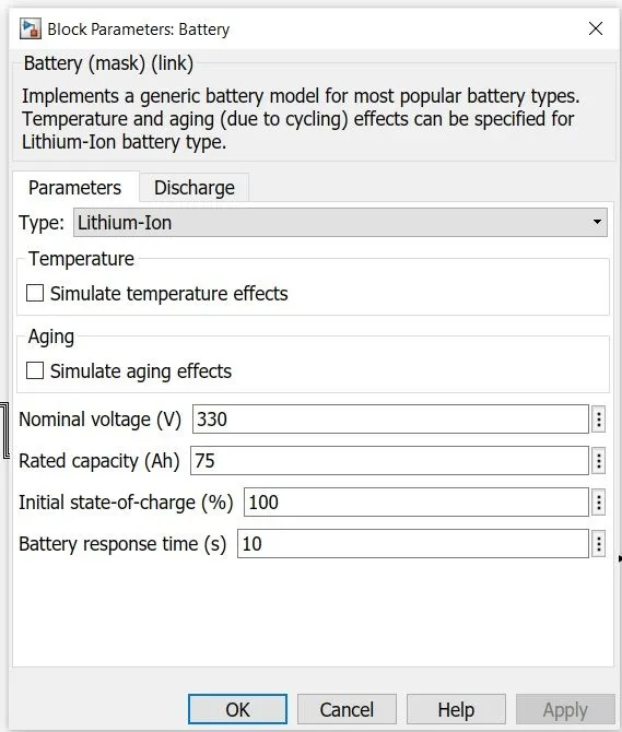
The Battery block implements a generic dynamic model that represents most popular types of rechargeable batteries.

This figure shows the equivalent circuit that the block models.

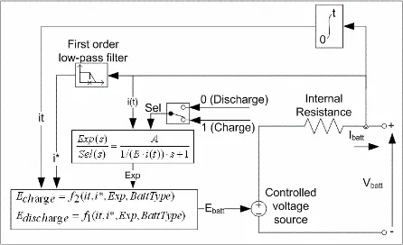
Charge and Discharge Characteristics

The circuit parameters can be modified to represent a specific battery type and its discharge characteristics. A typical discharge curve consists of three sections.

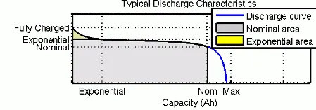
The first section represents the exponential voltage drop when the battery is charged. The width of the drop depends on the battery type. The second section represents the charge that can be extracted from the battery until the voltage drops below the battery nominal voltage. Finally, the third section represents the total discharge of the battery, when the voltage drops rapidly.

When the battery current is negative, the battery recharges, following a charge characteristic.

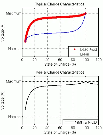
The model parameters are derived from the discharge characteristics. The discharging and charging characteristics are assumed to be the same.

The Exp(s) transfer function represents the hysteresis phenomenon for the lead-acid, nickel-cadmium (NiCD), and nickel-metal hydride (NiMH) batteries during the charge and discharge cycles. The exponential voltage increases when a battery is charging, regardless of the battery's state of charge. When the battery is discharging, the exponential voltage decreases immediately.

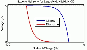
The state of charge (SOC) for a battery is a measure of battery's charge, expressed as a percent of the full charge. The depth of discharge (DOD) is the numerical compliment of the SOC, such that DOD = 100% - SOC.

For example, if the SOC is:

100% — The battery is fully charged and the DOD is 0%.
75% — The battery is 3/4 charged and the DOD is 25%.
50% — The battery is 1/2 charged and the DOD is 50%.
0% — The battery is has 0 charge and the DOD is 100%.

Model Validation

Experimental validation of the model shows a maximum error of 5% (when SOC is between 10% and 100%) for the charge (when the current is 0 through 2 C) and discharge (when the current is 0 through 5 C) dynamics.

Parameterization

Extract Battery Parameters from Data Sheets

This figure shows detailed parameters extracted from the Panasonic NiMH-HHR650D battery data sheet.

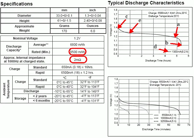
These parameters are approximate and depend on the precision of the points obtained from the discharge curve.

The discharge curves you obtain from these parameters, which are marked by dotted lines in the following figures, are similar to the data sheet curves.

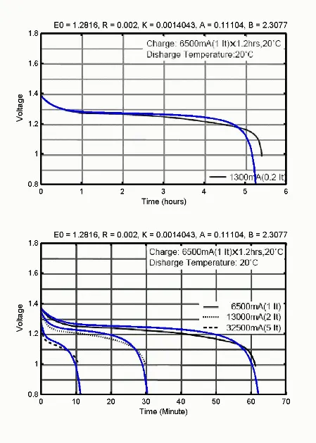
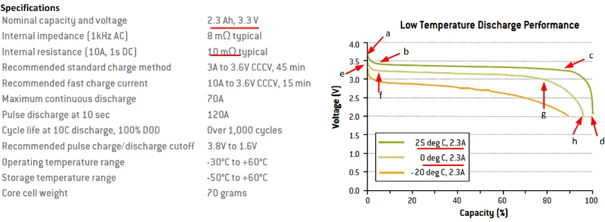
To represent the temperature effects of the lithium-ion (Li-ion) battery type, an additional discharge curve at ambient temperature, which is different from the nominal temperature, and the thermal response parameters are required. Additional discharge curves are not usually provided on the data sheet and may require simple experiments to be obtained. The following examples show parameters extracted from the A123 Li-iron-phosphate ANR26650M1 and the Panasonic Li-cobalt-oxide CGR 18,650 AF battery data sheets.

The A123 ANR26650M1 data sheet specifications include the required discharge curve points and other required parameters.

BUS SELECTOR:-

The Bus Selector block outputs the elements you select from the input bus. The block can output the selected elements separately or in a new virtual bus.

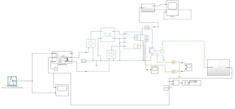
FOLLOWING ARE FIGURES FROM MATLAB PROGRAM THAT IS INCLUDED

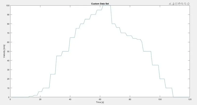
FOLLOWING FIGURE SHOWS THE INPUT FROM EXCEL SHEET THAT IS ALSO INCLUDED

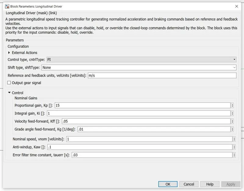
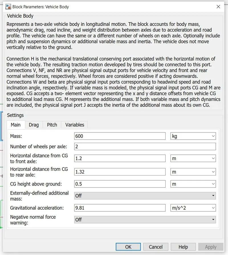
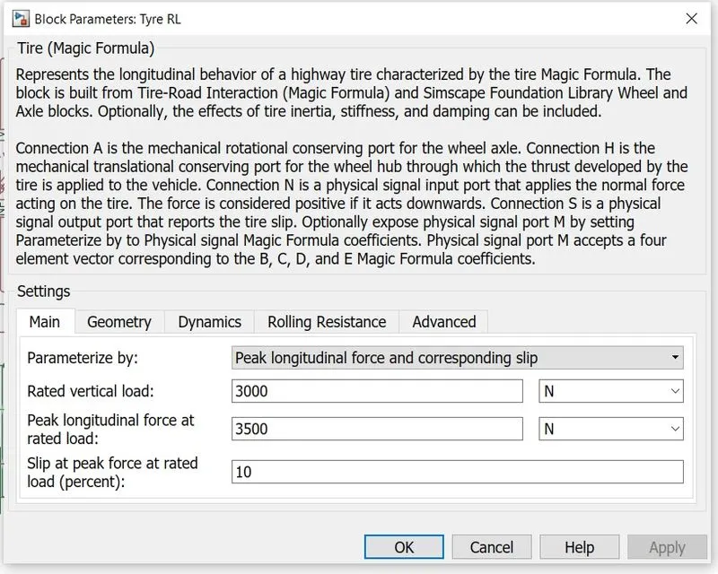
THE FOLLOWING FIGURE SHOWS VARIOUS PARAMETERS FOR ALL THE BLOCKS USED:-

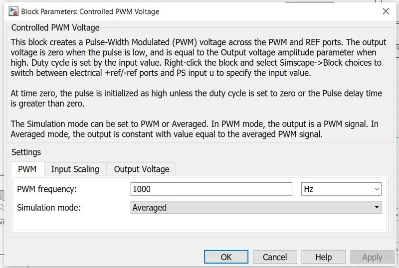
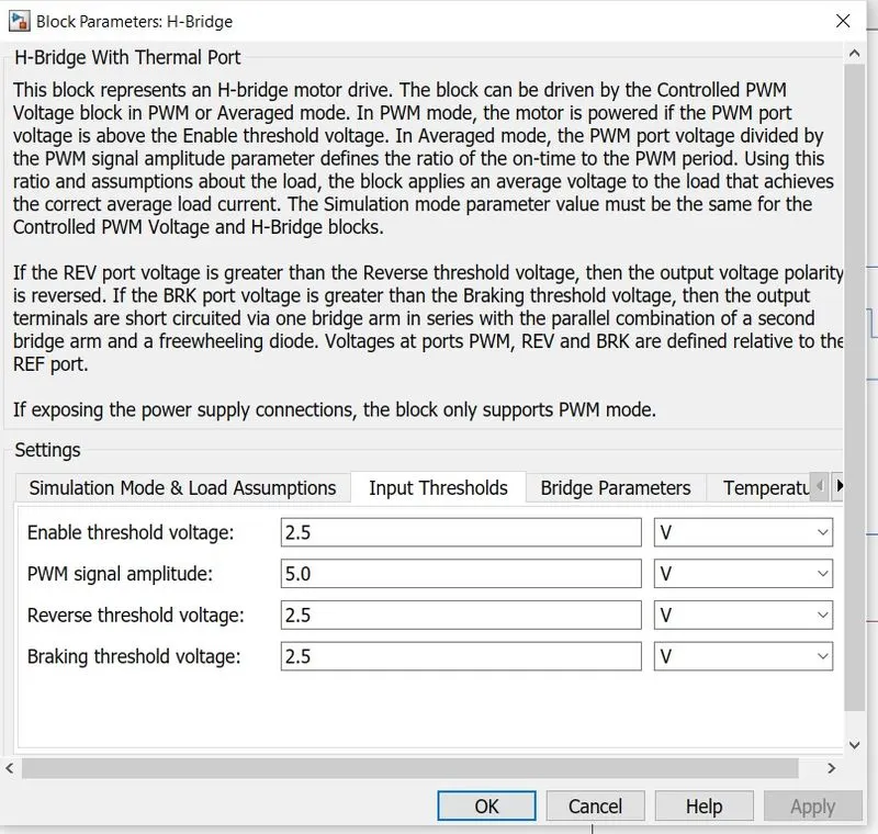
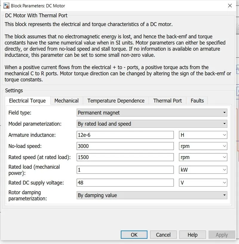
FOLLOWING FIGURE SHOWS THE SUB BLOCK FOR BATTERY AND SOC:-

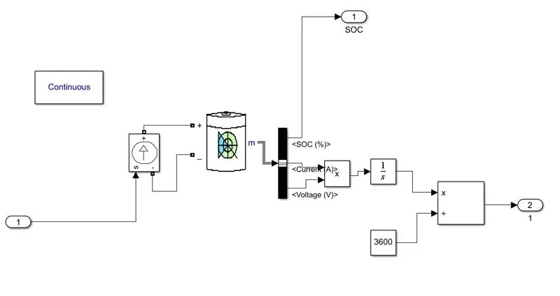
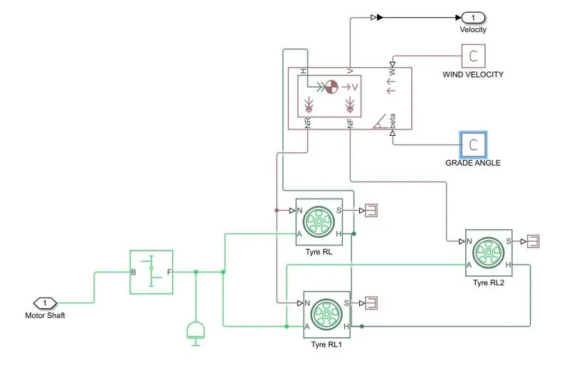
FOLLOWING BLOCK REPRESENTS THE MECHANICAL SIDE WITHIN A SUB BLOCK:-

RESULTS:-

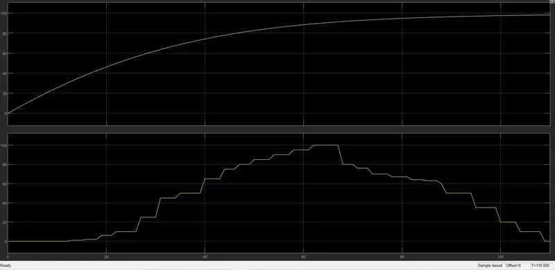
FROM THE ABOVE FIGURE WE CAN SEE THAT THERE IS A SLIGHT DROP IN SPEED IN THE ACTUAL OUTPUT VERSUS THE INPUT GIVEN FROM THE EXCEL SHEET. THE OUTPUT IS NOT MOVING UP AND DOWN AS IN THE EXCEL SHEET TO SOME EXTENT THAT THE MOMENTUM OF THE VEHICLE, SO THERE IS A SLIGHT DELAY FROM THE INPUT.