Electric Rickshaw modelling

Aim

To create a detailed matlab model of an electric rickshaw with following objectives.

• To model the vehicle with rear wheels driven by PM brushed type motor
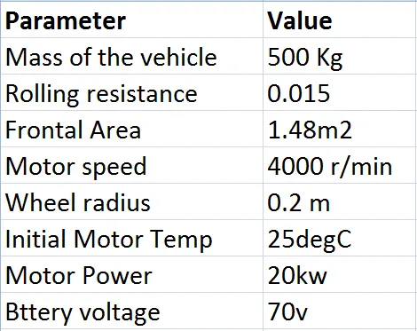
• Assume efficiency point of motor controller and make an excel sheet of all input and assumed data
• For any three standard driving cycles show energy consumption, temperature rise of motor controller for 100km constant speed driving at 45kmph.

Introduction

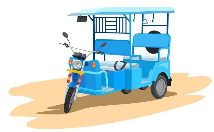
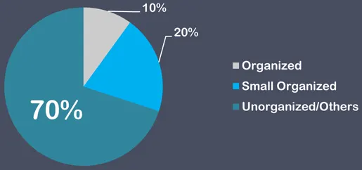
Electric rickshaws are becoming popular these days because of their low fuel cost, and less human effort compared to pulled rickshaws. They are being widely accepted as an alternative to petrol/diesel/CNG auto rickshaws. They are three-wheelers powered by an electric motor ranging from 650-1400 Watts. They are mostly manufactured in India and China. Battery run rickshaws could be a low emitter complementary transport for the low income people, who suffer most from a lack of transport facility, if introduced in a systematic manner. E-Rickshaw's have now transitioned from being a market entrant in the automobile segment of the country to evolve as a leading short distance transport solution. The share of production for e-rickshaws for now is indicated below.

These rickshaws have a mild Steel tubular chassis, consisting of three wheels with a differential mechanism at the rear wheels. The electrical system used in Indian version is 48V. Vehicles made in fibber are popular because of their strength and durability, resulting in low maintenance, especially in India. Body design is varied from load carriers, passenger vehicles with no roof, to full body with windshield for drivers comfort. It consists of a controller unit. They are sold on the basis of voltage supplied and current output, also the number of metal oxide field effect transistors used. The battery used is mostly lead acid battery with life of 6–12 months. Simple representation of the vehicle can be done by a block diagram and it is given below.

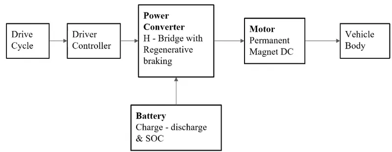
From the above diagram we will get a overall idea of the model of the vehicle. Now we can model the vehicle

Modelling and Explanation

The simulink model of the vehicle is represented below.

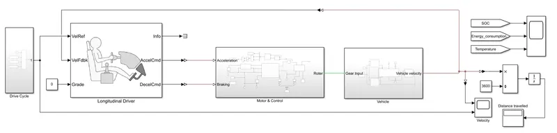
Firstly, the vehicle body was created and it was changed into a subsystem. Similarly, DC motor and related configurations were also created as a subsystem. Proper blocks were used to connect these and final model represented above was obtained.

→ Parameters and Specifications

Drive Cycle: Every vehicle needs a drive cycle so that we can simulate the performance. It will act as a drive input for the iterations. The drive cycle system which was created is given below.

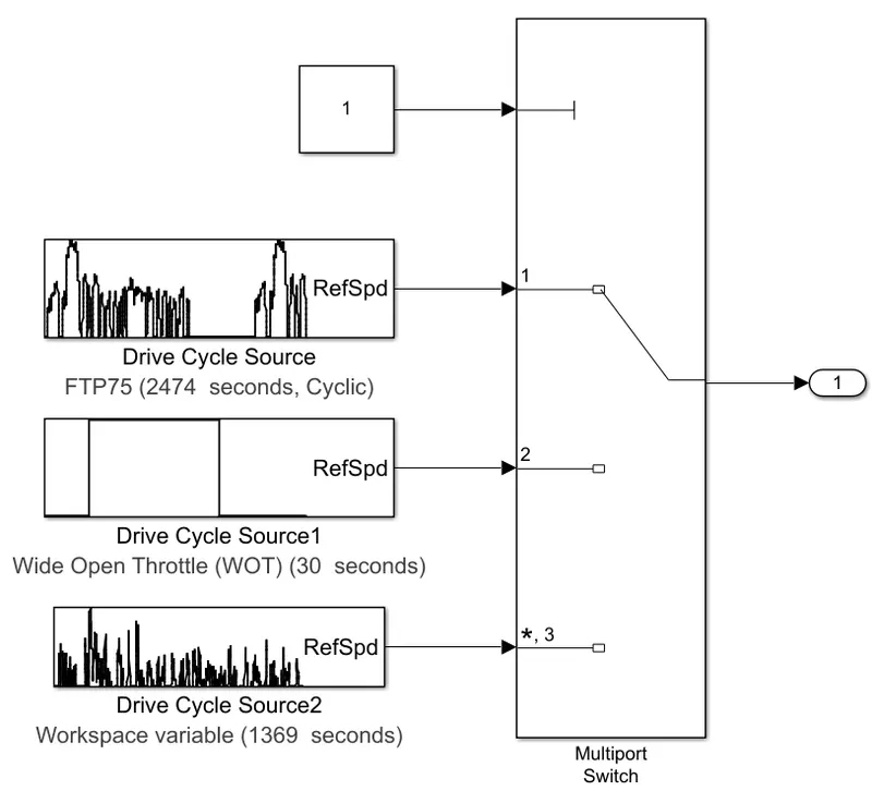
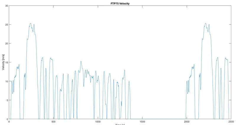
It consists of three drive cycle source. These blocks are connected to a multiport switch so that we can select one of them. Drive cycle source block generates a standard longitudinal drive cycle. The block output is the vehicle longitudinal speed. Here we have selected FTP75, UDDS and WOT Drive cycle for the simulation. Plot for the FTP75 cycle is given below.

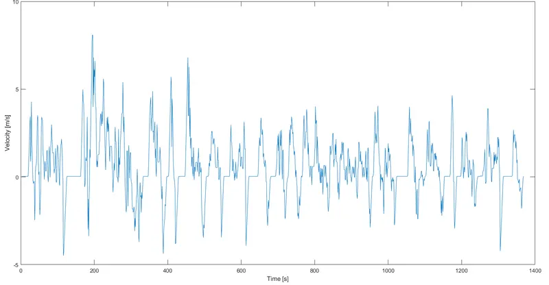
UDDS drive cycle is loaded from work space. Data of the cycle is stored in a excel sheet and it is loaded to workspace with import command.

Plot for the cycle is given below.

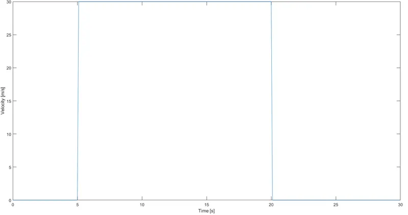
Default WOT cycle is given below.

Longitudinal Driver: It is a parametric longitudinal speed tracking controller for generating normalized acceleration and braking commands based on reference and feedback velocities. We have already given the reference velocity as drive cycle. In this block, we can add any grade values if we want. Acceleration and braking outputs is connected motor controlling unit.

Motor & Controller: This subsystem drives the shaft according to the input of driver. The representation of the subsystem is given below.

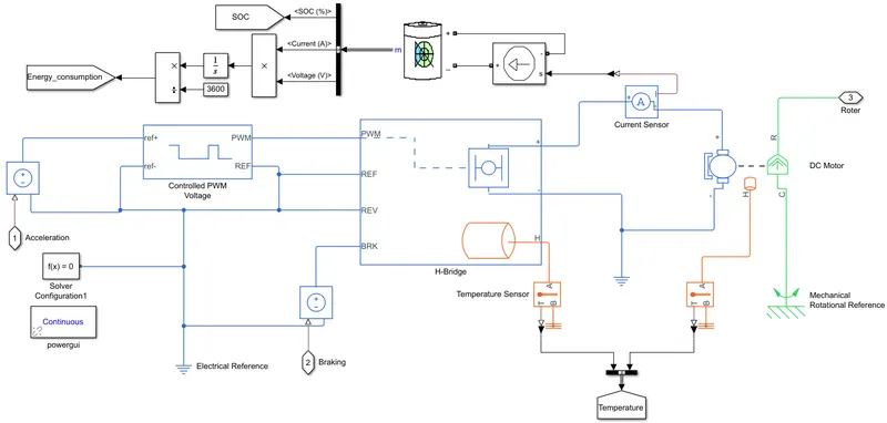
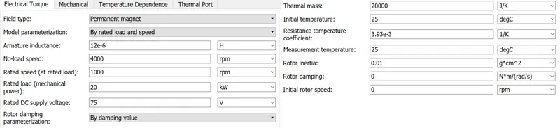
Here we used a DC motor to power the model. This block represents the electrical and torque characteristics of a DC motor. The block assumes that no electromagnetic energy is lost, and hence the back emf and torque constants have the same numerical value when in SI units. Motor parameters can either be specified directly, or derived from no load speed and stall torque. If no information is available on armature inductance, this parameter can be set to some small non zero value. The parameters given for motor are represented below.

DC motor is controlled by an H bridge block. Conditions for H bridge block are given below.

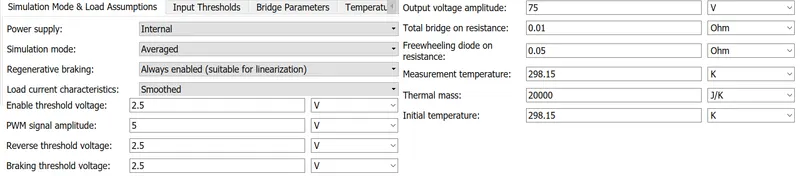
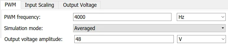
The block can be driven by the Controlled Pulse Width Modulator (PWM) Voltage block. We selected the average mode for PWM block. In Averaged mode, the PWM port voltage divided by the PWM signal amplitude parameter defines the ratio of the on-time to the PWM period. Using this ratio and assumptions about the load, the block applies an average voltage to the load that achieves the correct average load current. We kept the Simulation mode parameter value for the Controlled PWM Voltage and H-Bridge blocks same. If the REV port voltage is greater than the Reverse threshold voltage, then the output voltage polarity is reversed. If the BRK port voltage is greater than the Braking threshold voltage, then the output terminals are short circuited via one bridge arm in series with the parallel combination of a second bridge arm and a freewheeling diode. Voltages at ports PWM, REV and BRK are defined relative to the REF port. The PWM block will keep the output voltage zero when the pulse is low, and equal to the output voltage amplitude parameter when high. Parameters for PWM block are given below.

Duty cycle is set by the input value. A controlled current source is given to the modulator so that the power will not be used uncontrollably. Battery is also connected to the DC motor with a monitoring system for the battery. Specification for the battery is given below.

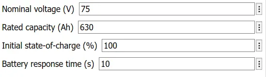
Temperature sensors are connected to DC motor and H Bridge for their temperature monitoring. This block measures temperature in a thermal network. Output results like temperature from sensor, soc and energy consumption from battery are connected to scope with from goto blocks.

Vehicle: This subsystem resembles the body of electric car and its representation is given below.

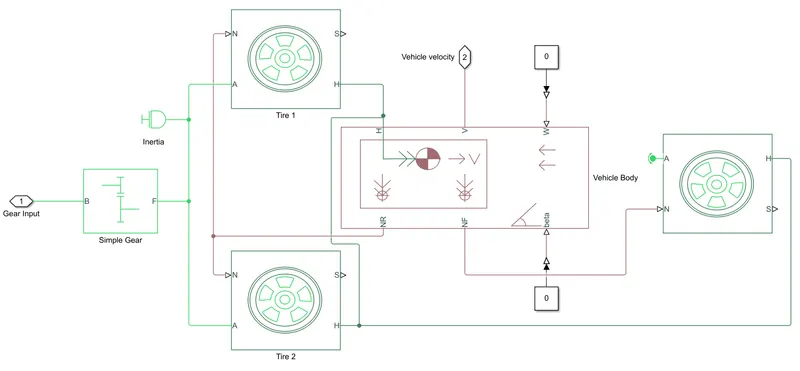
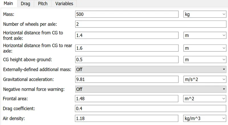
The vehicle body block represents a two-axle vehicle body in longitudinal motion. The block accounts for body mass, aerodynamic drag, road incline, and weight distribution between axles due to acceleration and road profile. Connection H is the mechanical translational conserving port associated with the horizontal motion of the vehicle body. The resulting traction motion developed by tires is connected to this port. Connections V, NF, and NR are physical signal output ports for vehicle velocity and front and rear normal wheel forces, respectively. Connections W and beta are physical signal input ports corresponding to wind speed and road inclination angle, respectively. The parameters for the block are given below.

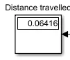
Gear input is given to the wheel blocks. We will get the vehicle velocity from the output port and it is given to the longitudinal driver block as feedback velocity. The feedback and reference velocities are connected to a scope block so that we can compare them. Output velocity is also integrated and converted to distance in kilometres by an integrator block.

Results

Simulation was done with the selected drive cycles and the results are shown below.

FTP75

The following plot shows the velocity plot of the vehicle. Red line is the reference drive cycle and blue one is the vehicle velocity.

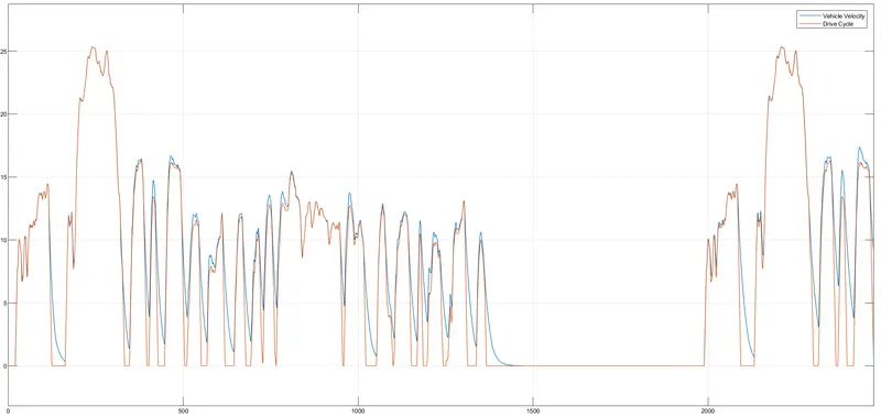
From the plot we can clearly see that the vehicle travelled according to our drive cycle. Maximum speed of the vehicle was same as the drive cycle and the distance travelled was also according to the cycle.

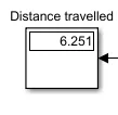
Now, we can look into the plot were the perfomance of the vehicle was analysed.

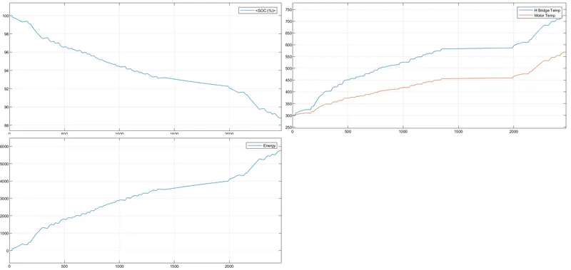
The first plot shows the SOC of the battery, second plot shows the temperature of DC motor and H bridge and third one energy consumed.

SOC of the battery dropped to 89% and energy consumption reached about 6000Wh. Motor temperature reached about 570K and controller temperature raised to about 725K.

UDDS

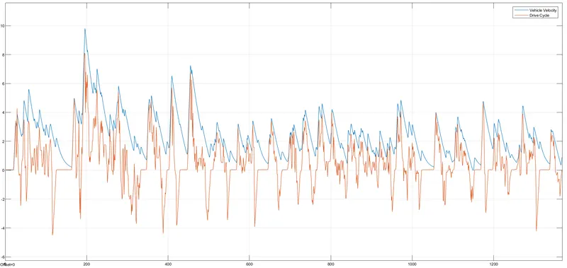
Here also the reference cycle and actual cycle overlapped each other and it is represented below.

Perfomance plots are given below.

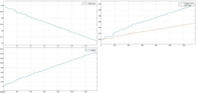
SOC of the battery dropped to 97% and energy consumption reached about 1450Wh. Motor temperature reached about 380K and controller temperature raised to about 420K.

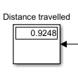
WOT

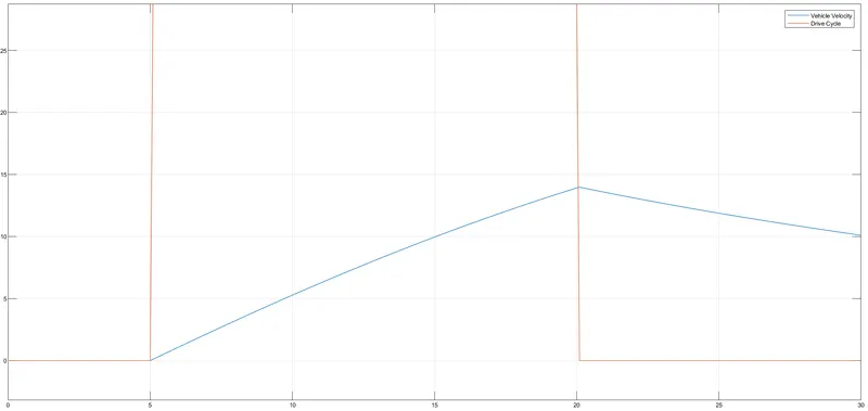
The vehicle velocity plot is given below.

Cycle is for 30 seconds and the perfomance for that time is given below.

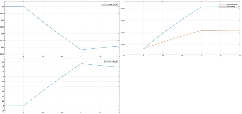
SOC of the battery dropped to 99.7% and energy consumption reached about 160Wh. Motor temperature reached about 305K and controller temperature raised to about 315K.

Conclusion

The vehicle model was created in matlab and simulation was done. In real life conditions, the temperature wont go as this much as we didnt included the cooling system and optimum parameters. Efficiency of the vehicle can be increased by optimising the battery, motor, vehicle body and controlling parameters. This model can be used as a reference for creating a real life model. Because the model gives results which is similar to theoretical values. Like the drive cycle of FTP is almost similar as vehicle speed. We can run the cycle repeatedly for more time until battery drains out to find out the maximum capacity so that the value will be more practical. As the result is feasible for one cycle we can calculate further with this reference.

Reference

[1] Modelling design and control of a light electric vehicle with hybrid energy storage system for Indian driving cycle, S Devi Vidhya and M Balaji, Measurement and Control 2019, Vol. 52(9-10) 1420–1433