Final Project: Electric Rickshaw modelling

Aim:

The main aim is to model an Electric Rickshaw using Simulink.

Objective:

The main objective is as follows:

1. The Rickshaw is a rear-wheel-drive by a PM brushed type motor.
2. Assuming the Efficiency points of the motor controller and motor.
3. Making an excel Sheet of all the input and assumed data.

Theory:

Electric Rickshaw:

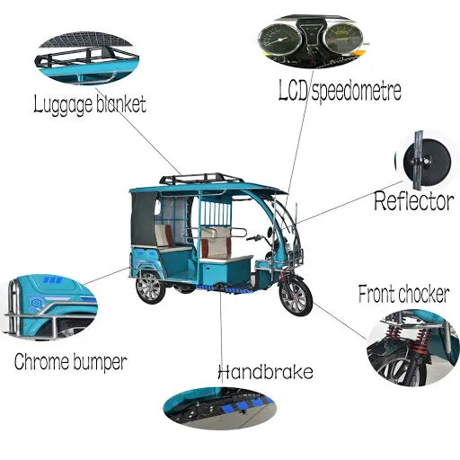
An auto-rickshaw is a motorized version of the pulled rickshaw or cycle rickshaw. There are many different auto rickshaw designs. The most common type is characterized by a sheet-metal body or open-frame resting on three wheels; a canvas roof with drop-down side curtains; a small cabin at the front for the driver, with handlebar controls; and a cargo, passenger, or dual-purpose space at the rear. Another common type is a motorcycle that has an expanded sidecar or, less often, is pushing or pulling a passenger compartment.

Electric rickshaws have been becoming more popular in some cities since 2008 as an alternative to auto rickshaws and pulled rickshaws because of their low fuel cost, and less human effort compared to pulled rickshaws. They are being widely accepted as an alternative to petrol/diesel/CNG auto-rickshaws. They are three-wheelers powered by an electric motor ranging from 650 to 1400 Watts. They are mostly manufactured in India and China, only a few other countries manufacture these vehicles. Battery-run rickshaws could be a low-emitter complimentary transport for the low-income people, who suffer most from a lack of transport facility if introduced systematically according to experts.

Procedure:

1. Creating the Vehicle Body:

Tire (Magic formula):

• We design the basic vehicle part that is tires, body, gear,
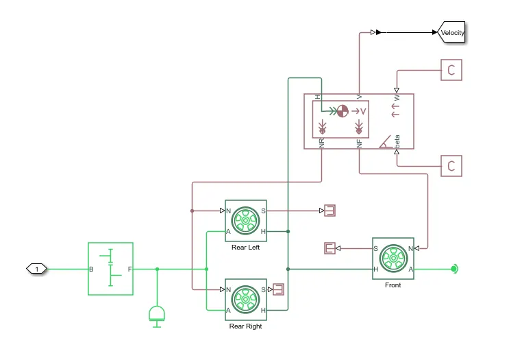
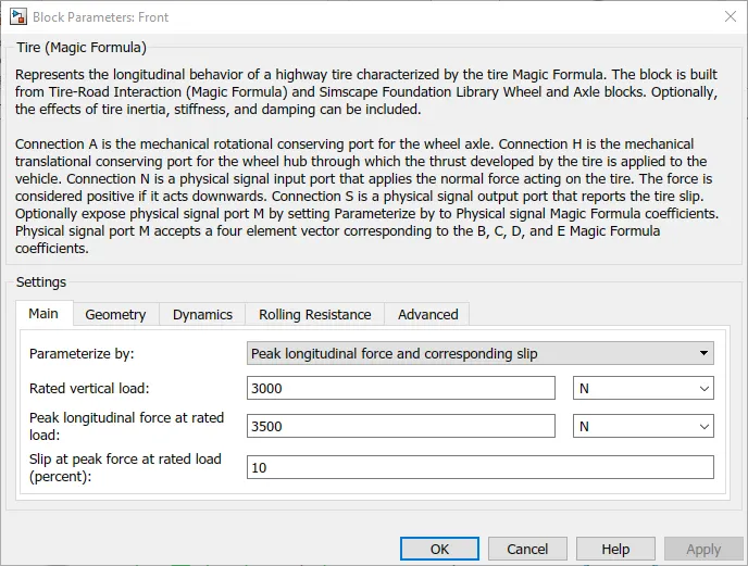
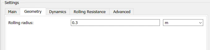
• First, we need to retrieve the Tires block named tire (magic formula). It represents the longitudinal behavior of a highway tire characterized by the tire Magic Formula. The block is built from Tire-Road Interaction (Magic Formula) and Simscape Foundation Library Wheel and Axle blocks. Optionally, the effects of tire inertia, stiffness, and damping can be included.
• The Tire has 4 connections, N (A physical Signal input port that applies the normal force acting on the tire), A ( The mechanical rotational conserving port for the Wheel axle), H (A mechanical translational conserving port for the wheel hub through which the thrust developed by the tire is applied to the vehicle), and S (A physical signal output port that reports the tire slip).
• Now, Connect the H-port to all the other H-ports and connect the front A ports (Left and Right wheels) with each other and Rear with each other.
• Connect the N ports of the tires to the front left tire and Front right tire. And connect N ports of the rear left to the rear right.

Vehicle Body:

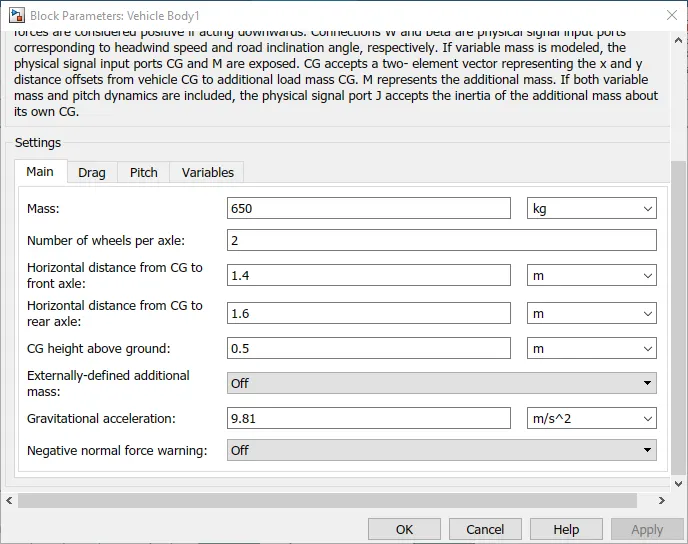
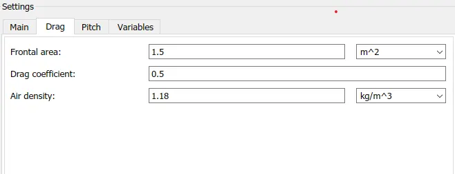
Connection H is the mechanical translational conserving port associated with the horizontal motion of the vehicle body. The resulting traction motion developed by tires should be connected to this port. Connections V, NF, and NR are physical signal output ports for vehicle velocity and front and rear normal wheel forces, respectively. Wheel forces are considered positive if acting downwards. Connections W and beta are physical signal input ports corresponding to headwind speed and road inclination angle, respectively. If the variable mass is modeled, the physical signal input ports CG and M are exposed. CG accepts a two-element vector representing the x and y distance offsets from vehicle CG to additional load mass CG. M represents the additional mass. If both variable mass and pitch dynamics are included, the physical signal port J accepts the inertia of the additional mass about its own CG.

• Create a Vehicle body block and attach the NF port to the front end (Front tires) of the N- ports and attach the NR port to the Rear end (Rear Tires) of the N-ports.
• Create a physical constant block to attach it to the beta and W ports. Since we are not considering the hill-climbing ascent and the Wind speed.
• Connect the H-port of the Vehicle Body block to the H ports of the tire.
• Connect the V port of the Vehicle body block to the ‘Go to’ block naming it as Velocity via PS- Simulink converter.

Simple Gear:

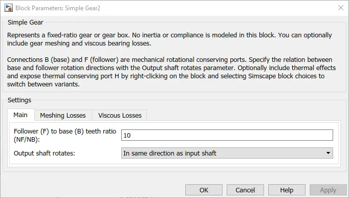
It represents a fixed-ratio gear or gearbox. No inertia or compliance is modeled in this block. You can optionally include gear meshing and viscous bearing losses. Connections B (base) and F (follower) are mechanical rotational conserving ports. Specify the relation between base and follower rotation directions with the Output shaft rotates parameter. Optionally include thermal effects and expose thermal conserving port H by right-clicking on the block and selecting Simscape block choices to switch between variants.

• Connect the F-port of the Simple Gear to the Axles i.e. A- ports of the rear tires making it a Rear Wheel Drive.
• Also, connect the inertia block to the F- port of the Simple Gear.
• Keep the B- port of the extended.
• Now, Select the Parts creating the box and create a subsystem and name it as Vehicle Body.
• Now create a simple DC motor block and connect the R- port to the Extended B- port.

DC Motor:

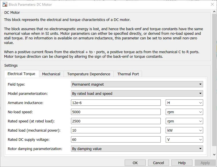
The DC Motor block represents the electrical and torque characteristics of a DC motor.

The block assumes that no electromagnetic energy is lost, and hence the back EMF and torque constants have the same numerical value when in SI units. Motor parameters can either be specified directly or derived from the no-load speed and stall torque. If no information is available on armature inductance, this parameter can be set to some small non-zero value.

When a positive current flows from the electrical + to - ports, a positive torque acts from the mechanical C to R ports. Motor torque direction can be changed by altering the sign of the back-EMF or torque constants.

2. Creating the Power Source Block:

H-Bridge:

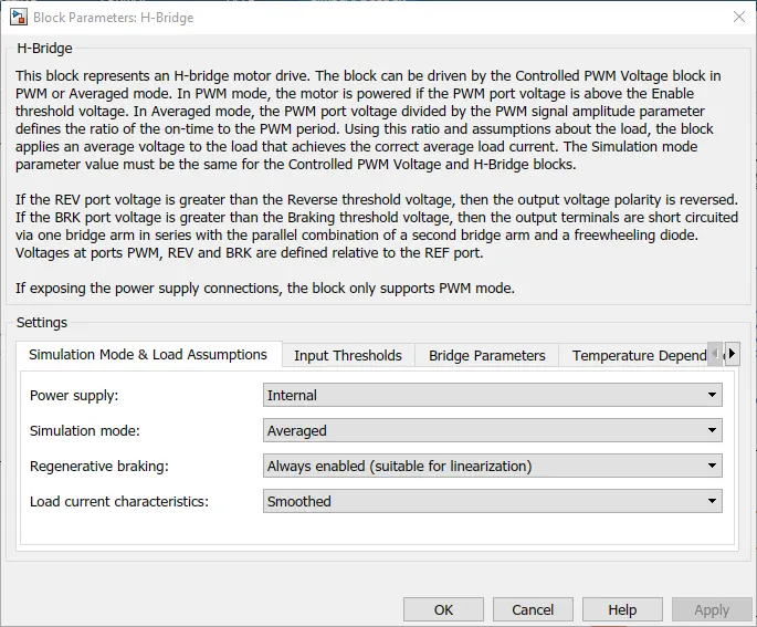
This block represents an H-bridge motor drive. The block can be driven by the Controlled PWM Voltage block in PWM or Averaged mode. In PWM mode, the motor is powered if the PWM port voltage is above the Enable threshold voltage. In Averaged mode, the PWM port voltage divided by the PWM signal amplitude parameter defines the ratio of the on-time to the PWM period. Using this ratio and assumptions about the load, the block applies an average voltage to the load that achieves the correct average load current. The Simulation mode parameter value must be the same for the Controlled PWM Voltage and H-Bridge blocks.

If the REV port voltage is greater than the Reverse threshold voltage, then the output voltage polarity is reversed. If the BRK port voltage is greater than the Braking threshold voltage, then the output terminals are short-circuited via one bridge arm in series with the parallel combination of a second bridge arm and a freewheeling diode. Voltages at ports PWM, REV, and BRK are defined relative to the REF port.

If exposing the power supply connections, the block only supports PWM mode.

• Create an H-bridge block and double click on it and change the Simulation mode to Averaged.
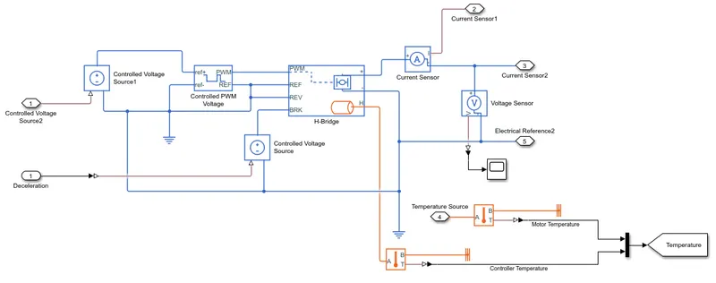
• Create the Current sensor block and connect the positive port to the positive port of the H-Bridge. And negative port to the positive port of the DC motor. I- port is extended to make a connection afterward.
• The REV and REF of the H-bridge are connected to the Solver Configuration.
• BRK (Brake) port is connected to the positive port of the Controlled Voltage Source. And the Negative Port is connected to the negative port of the H-Bridge which is connected to an Electrical Reference that in return is connected to the DC motor negative port.

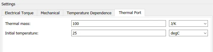
The Thermal Port is initially hidden. We need to unhide it by right-clicking on the block >> select the Simscape option >> Select Block choices >> Select ‘Show Thermal ports’.

Now, Open the H-Bridge block and go to the thermal ports and change the Thermal Mass to 4500 J/K.

Controlled PVM Voltage:

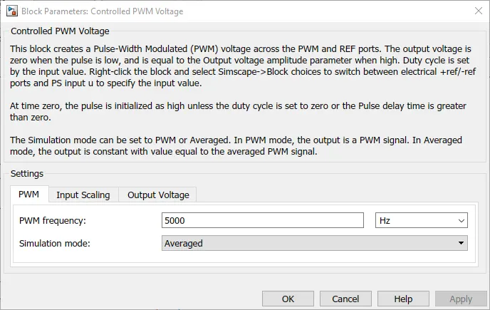
The duty cycle is set by the input value. Right-click the block and select Simscape Block choices to switch between electrical +ref/-ref ports and PS input u to specify the input value. At time zero, the pulse is initialized as high unless the duty cycle is set to zero or the Pulse delay time is greater than zero. The Simulation mode can be set to PWM or Averaged. In PWM mode, the output is a PWM signal. In Averaged mode, the output is constant with a value equal to the averaged PWM signal.

• The PVM port of the Controlled PVM Voltage to the PVM port of the H-Bridge and the REF port to the REF and REV port of the H-bridge.
• Connect the positive port of the Controlled Voltage Source to the ‘ref +’ and the Negative port is connected to the ‘ref –’ along with the electrical reference.
• The physical signal is extended.
• Select all the blocks and create a subsystem named Power Source Unit.

3. Create a Longitudinal Driver Block:

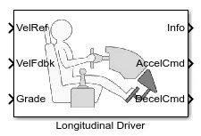
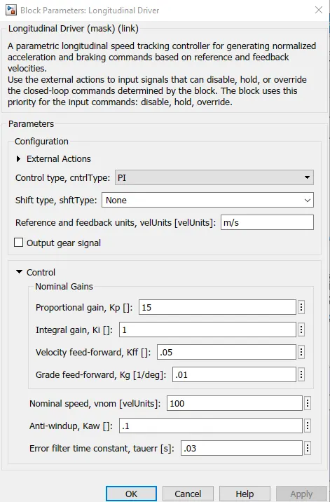
A parametric longitudinal speed tracking controller for generating normalized acceleration and braking commands based on reference and feedback velocities. Use the external actions to input signals that can disable, hold, or override the closed-loop commands determined by the block. The block uses this priority for the input commands: disable, hold, and override.

• Create a longitudinal driver block and connect the “AccelCmd” to the physical signal of the controlled voltage of the power unit.
• Connect the ‘DecelCmd’ to the physical signal of the other controlled voltage source.
• Create a constant as ‘0’ to Grade.

4. Creating the Battery Unit and State of Charge (SOC) Unit:

Battery:

This block models a battery. The block models the battery as a series internal resistance and a constant voltage source if you select Infinite for the Battery charge capacity parameter. If you select Finite for the Battery charge capacity parameter, the block models the battery as a series internal resistance plus a charge-dependent voltage source defined by:

Where SOC is the state of charge and is the nominal voltage. Coefficient beta is calculated to satisfy a user-defined data point [AH1, V1].

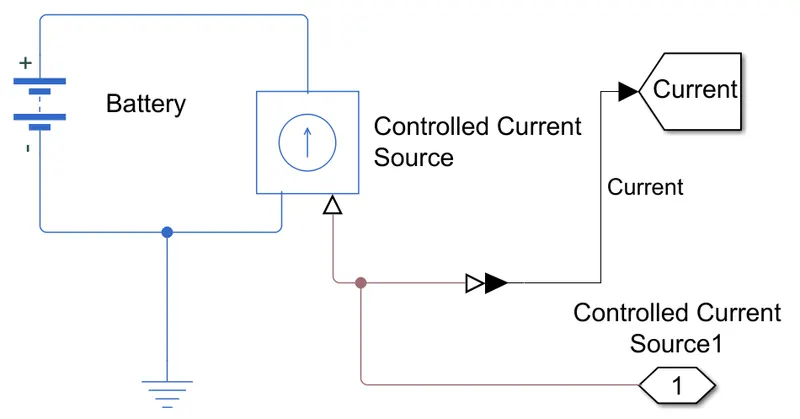
• The positive terminal of the battery is connected to the positive port of the Controlled Current Source and the negative terminal to the negative port of the controlled current source via electrical reference.
• The Physical signal of the current source is connected to PS- Simulink Converter to connect the ‘Go to’ block namely the current.
• Select the blocks and create a subsystem naming it as Battery.
• The current sensor ‘I’ which we extended earlier is connected to the Physical signal of the controlled current source.
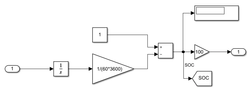
• Now, connect the Ps- Simulink to the Integrator and connect the integrator to the Gain such that the ampere-hour is converted to ampere sec, and connect it to the sum block with the constant of 1.
• Connect the Sum block to the multiply block of 100.
• Create a ‘Go to’ block and name it SOC and connect to the Sum of the Integrator block.
• Select the Blocks and create a subsystem and name it as SOC.

Battery Subsystem:

SOC Subsystem:

5. Giving the Drive Cycle Input:

It generates a standard or user-specified longitudinal drive cycle. The block output is the vehicle's longitudinal speed. Use the fault tracking parameters to identify drive cycle faults within the specified speed and time tolerances.

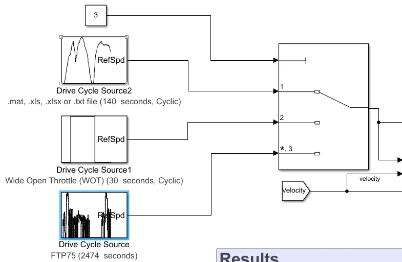
• Open the Drive cycle source and select the Drive cycle as ‘FTP75’ and click ok.
• Connect the ‘Refspd’ to the ‘Velref’ of the longitudinal Drive block.
• Create the ‘From’ block and connect it to the ‘VelFdbk’.
• Connect the ‘from velocity’ block to the Multiport Switch which is then connected to the MUX along with the drive cycle and the ‘Go to’ Block is created and connected to the output of the MUX.
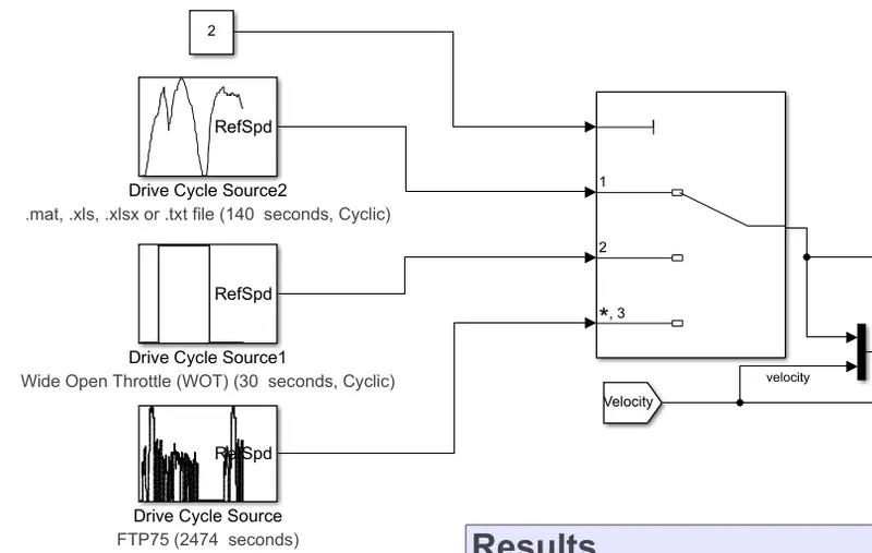
• Use a new Drive Cycle Source and change the drive cycle source to Wide Open Throttle (WOT). Change the nominal reference speed to 45 and click on apply.
• For the third Drive Cycle, create an excel sheet showing the Time and Speed for 140 seconds. Import the file in the drive cycle source.
• The multiport input is initially given as 3 in the constant block.

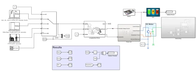
Final Model:

Results:

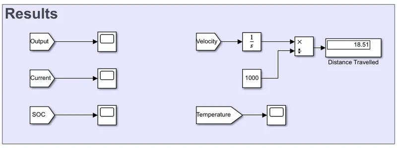
First considering the Output Speed, Temperature, Current, and SOC for the 3 Different Types of Drive Cycle we see the plot for different drive cycles mentioned below.

Drive Cycle FTP75:

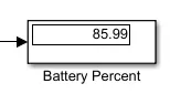
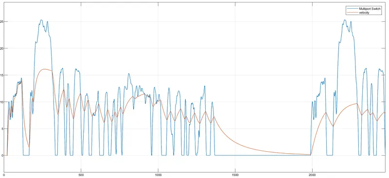
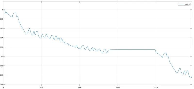
After the model is simulated, we can see that the distance traveled is 18.51 km and have a battery percent of 85.99%.

Battery Percent:

Output Speed:

In the output speed plot, it can be seen that the Drive Cycle speed and Velocity by the vehicle plots. The Velocity tries to achieve the drive train source parameters but tries to attain the velocity at the peak at 16 m/s.

Current:

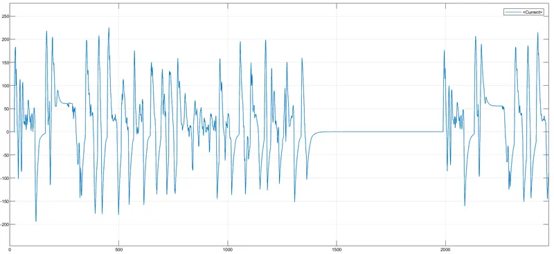
In the current plot, initially, there’s a noise but it settles within the range of +100 to -100. It can be reduced if we can go to the PID controller instead of the Longitudinal Driver.

SOC:

In the State of Charge plot, the battery starts with 100% but gradually reduces to 85.99% at the end of the cycle.

Temperature:

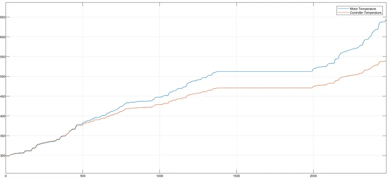
In the temperature plot, the motor and controller temperature increase to a temperature of around 650K and 550K approximately. It’s a Suitable temperature range.

WOT (Wide Open Throttle):

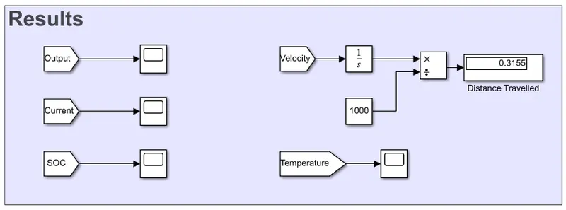
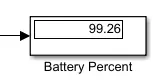
After the model is simulated, we can see that the distance traveled is 0.3155 km and the battery percent is reduced to 99.26% for the time of 30 seconds

Battery percent:

Output Speed:

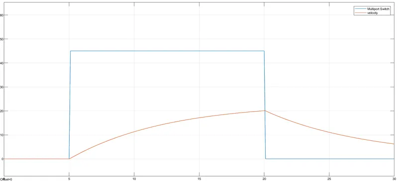
In the output speed plot, it can be seen that the Drive Cycle speed and Velocity by the vehicle plots. The Velocity tries to achieve the drive train source parameters but tries to attain the velocity at the peak at 20 m/s.

Current:

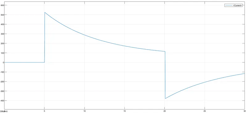
The current in this plot increases and there is a sharp reduction in the current and then it increases gradually.

SOC:

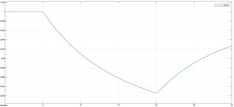
In the State of Charge plot, the battery starts with 100% but gradually reduces to 98.24% at the 20^th second and increases by the end of the cycle.

Temperature:

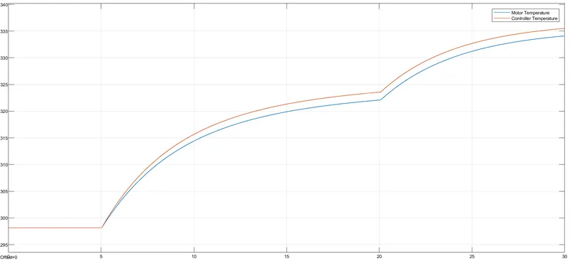
In the temperature plot, the motor and controller temperature increase to a temperature of around 336K and 334K approximately. It’s a Suitable temperature range.

Drive Cycle using the excel sheet:

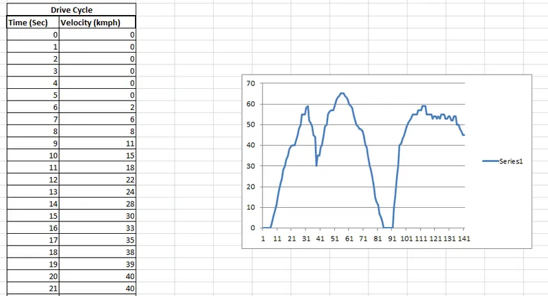
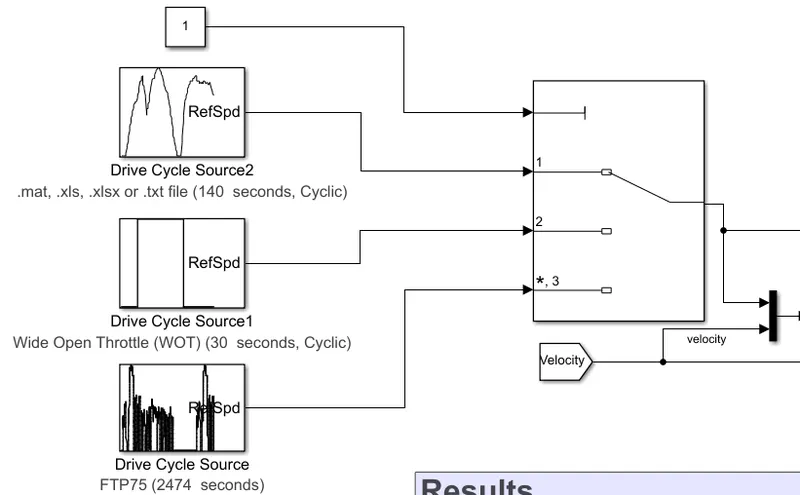
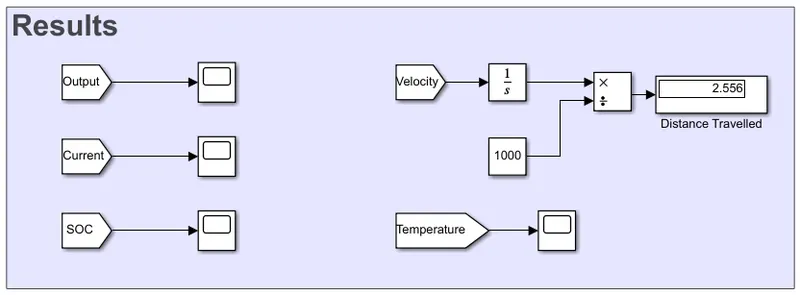
After the model is simulated, we can see that the distance traveled is 2.556 km and have a battery percent of 95.36%.

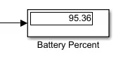
Battery Percent:

Output Speed:

In the output speed plot, it can be seen that the Drive Cycle speed and Velocity by the vehicle plots. The Velocity tries to achieve the drive train source parameters but tries to attain the velocity at the peak at 24 m/s and then it decreases and then it increases again just to maintain the steady-state.

Current:

In the current plot, The current flow is stable but it rapidly decreases and maintains, and then it decreases again, and then it increases.

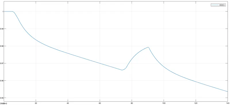
SOC:

In the State of Charge plot, the battery starts with 100% but gradually reduces to 95.36% at the end of the cycle.

Temperature:

In the temperature plot, the motor and controller temperature reaches a similar temperature of 360K. It’s a Suitable temperature range for the motor and controller.

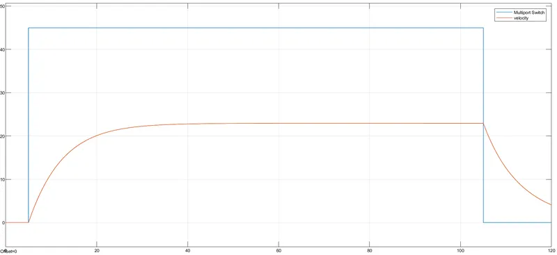
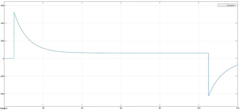
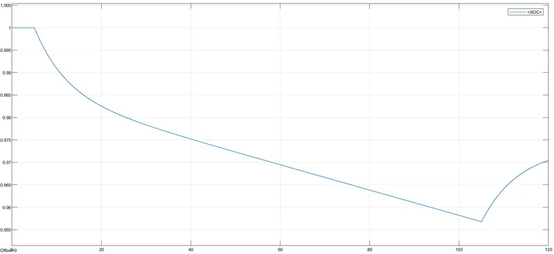
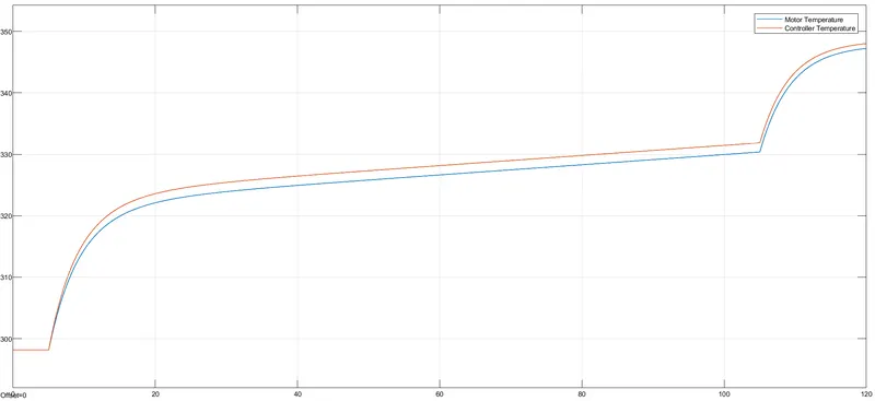
Drive Cycle for a constant speed of 45 KMPH for 100km:

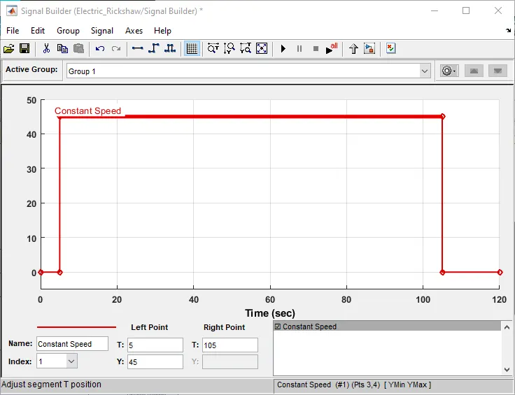
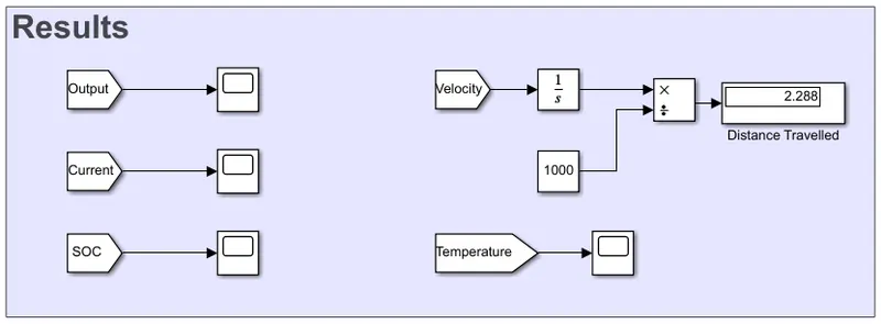
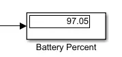
After the model is simulated, we can see that the distance traveled is 2.288 km and have a battery percent of 97.05%.

Battery Percent:

Output Speed:

In the output speed plot, it can be seen that the Drive Cycle speed and Velocity by the vehicle plots. The Velocity tries to achieve the drive train source parameters but tries to attain the velocity at the peak at 22 m/s and attains a steady-state and then it decreases to 0 when the Drive Cycle ends.

Current:

In the current plot, the current increase at 5 sec, and then it reaches a steady state.

SOC:

In the State of Charge plot, the battery starts with 100% but gradually reduces to 97.05% at the end of the cycle.

Temperature:

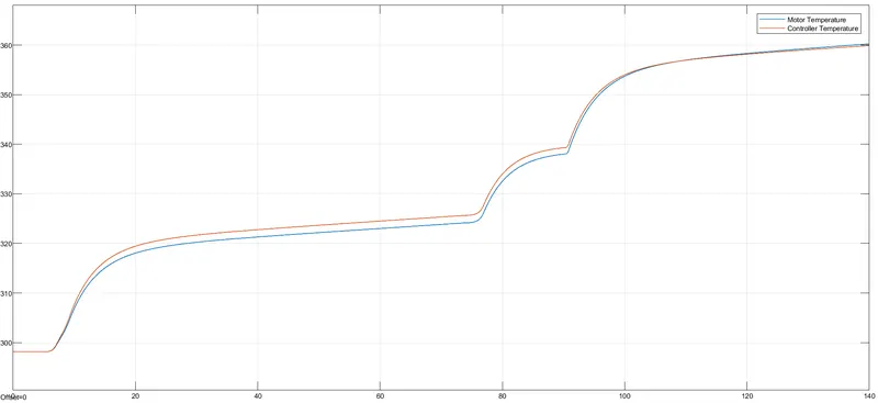
In the temperature plot, the motor and controller temperature reaches a similar temperature of 348K and 347.5K. It’s a Suitable temperature range for the motor and controller.

Tools Used:

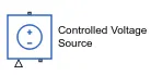
1. Controlled Voltage Source:

The Controlled Voltage Source block represents an ideal voltage source that is powerful enough to maintain the specified voltage at its output regardless of the current passing through it. The output voltage is V = Vs, where Vs is the numerical value presented at the physical signal port.

2. Controlled Current Source:

The Controlled Current Source block represents an ideal current source that is powerful enough to maintain the specified current through it regardless of the voltage across it. The output current is I = Is, where the numerical value is presented at the physical signal port.

3. Current Sensor:

The Current Sensor block represents an ideal current sensor, a device that converts current measured in any electrical branch into a physical signal proportional to the current.

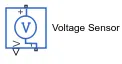
4. Voltage Sensor:

The Voltage Sensor block represents an ideal voltage sensor, a device that converts voltage measured between any electrical connections into a physical signal proportional to the voltage.

5. Integrator:

It is a Continuous-time integration of the input signal. An integrator in measurement and control applications is an element whose output signal is the time integral of its input signal. It accumulates the input quantity over a defined time to produce a representative output.

6. Temperature Sensor:

The Temperature Sensor block measures temperature in a thermal network. There is no heat flow through the sensor. The physical signal port T reports the temperature difference across the sensor. The measurement is positive when the temperature at port A is greater than the temperature at port B.