Final Project: Electric Rickshaw modelling
Aim: To model and simulate Electric Rickshaw.
Objective: • Rear-wheel drive-by PM brushed type motor. • Simulation for three drive cycles. • Energy consumption, temperature rise and controller parameters to be display as a result.
Theory:
Introduction:
Electric rickshaws have been becoming more popular in some cities since 2008 as an alternative to auto rickshaws and pulled rickshaws because of their low fuel cost, and less human effort compared to pulled rickshaws. They are being widely accepted as an alternative to petroVdieseVCNG auto-rickshaws.
They are three-wheelers powered by an electric motor ranging from 650 to 1400 Watts. They are mostly manufactured in India and China, only a few other countries manufacture these vehicles.
Battery-run rickshaws could be a low-emitter complimentary transport for the low-income people, who suffer most from a lack of transport facility if introduced in a systematic manner according to experts.
Design and construction: These rickshaws have an M.S(Mild Steel) tubular Chassis, consisting of three wheels with a differential mechanism the rear wheels. The motor is a brushless DC motor manufactured mostly in India and China. The electrical system used in the Indian version is 48V and in Bangladesh is 60V. The body design from the most popular Chinese version is of very thin iron or aluminium sheets. Vehicles made in fibre are also popular because of their strength and durability, resulting in low maintenance, especially in India. The body design is varied from load carriers, passenger vehicles with no roof, to full body with windshield for drivers comfort. It consists of a controller unit. They are sold on the basis of voltage supplied and current output, also the number of MOSFET (metal oxide field-effect transistors) used. The battery used is mostly a lead-acid battery with a life of 6-12 months. Deep cycle batteries designed for electric vehicles are rarely used. The weight of the electric car has also been a recurring design difficulty in them.
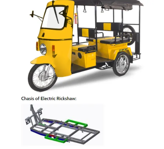
Specifications: • MAX. SPEED<25Kmph
• MILEAGE 100 Km
• SEATING/LOAD CAPACITYD.4 Passenger/40 Kg
• BATTERY CAPACITY100 Ah
• BATTERY TYPELead Acid Battery
• TYRE (F.12)3x17", 6PR
• MTOR TYPEBLDC Direct Drive Motor
• MOTOR INPUT VOLTAGE48V DC
• BRAKE (FAR) 130 mm Dia (Drum Type)
• CHARGERCompact & Easy to use 48V-12A/15,3-Stages SMPS Charger
• SPEEDOMETERAnalog
• STARTING SYSTEMElectric Start
• FRONT SHOCK ABSORBERHydraulic (Telescopic Type)
• REAR SHOCK ABSORBERLeaf Spring . Hydraulic (Telescopic Type) With Spring
• CHASSIS TYPESheet Metal, Spoke Type
• GROSS VEHICLE WEIGHTComfort 735 Kg
Dimensions:
• LXWX H2790 X 1000 X 1800 mm
• WHEEL BASE 1780 mm
• TURNING RADIUS 2755 mm
• GROUND CLEARANCE235 mm
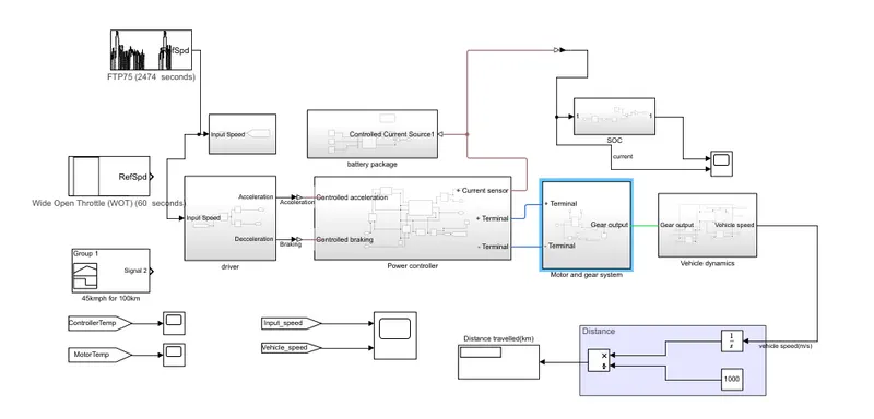
Matlab model of Electric Rickshaw:
Tire (Magic Formula):-
Description
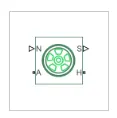
The Tire (Magic Formula) block models a tire with longitudinal behavior given by the Magic Formula [1], an empirical equation based on four fitting coefficients. The block can model tire dynamics under constant or variable pavement conditions.
The longitudinal direction of the tire is the same as its direction of motion as it rolls on pavement. This block is a structural component based on the Tire-Road Interaction (Magic Formula) block.
To increase the fidelity of the tire model, you can specify properties such as tire compliance, inertia, and rolling resistance. However, these properties increase the complexity of the tire model and can slow down simulation. Consider ignoring tire compliance and inertia if simulating the model in real time or if preparing the model for hardware-in-the-loop (HIL) simulation.
Tire Model
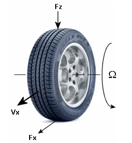
The Tire (Magic Formula) block models the tire as a rigid wheel-tire combination in contact with the road and subject to slip. When torque is applied to the wheel axle, the tire pushes on the ground (while subject to contact friction) and transfers the resulting reaction as a force back on the wheel. This action pushes the wheel forward or backward. If you include the optional tire compliance, the tire also flexibly deforms under load.
The figure shows the forces acting on the tire. The table defines the tire model variables.
Vehicle Body:-
Two-axle vehicle with longitudinal dynamics and motion and adjustable mass, geometry, and drag propertiesexpand all in page
Description
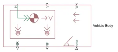
The Vehicle Body block represents a two-axle vehicle body in longitudinal motion. The vehicle can have the same or a different number of wheels on each axle. For example, two wheels on the front axle and one wheel on the rear axle. The vehicle wheels are assumed identical in size. The vehicle can also have a center of gravity (CG) that is at or below the plane of travel.
The block accounts for body mass, aerodynamic drag, road incline, and weight distribution between axles due to acceleration and road profile. Optionally include pitch and suspension dynamics. The vehicle does not move vertically relative to the ground.
The block has an option to include an externally-defined mass and an externally-defined inertia. The mass, inertia, and center of gravity of the vehicle body can vary over the course of simulation in response to system changes.
Model
The vehicle axles are parallel and form a plane. The longitudinal, x, direction lies in this plane and perpendicular to the axles. If the vehicle is traveling on an incline slope, β, the normal, z, direction is not parallel to gravity but is always perpendicular to the axle-longitudinal plane.
Input ports: • W - Headwind speed (m/s)
• beta - Road incline angle(rad)
• CG - Centre of gravity(m)
• M - Mass(kg)
• J - External moment of inertia(kg*m^2)
Output ports:
• V - Longitudinal velocity(m/s)
• NF - Front axle normal force(N)
• NR - Rear axle normal force(N)
Conserving port:
• H - Horizontal motion
DC Motor:-
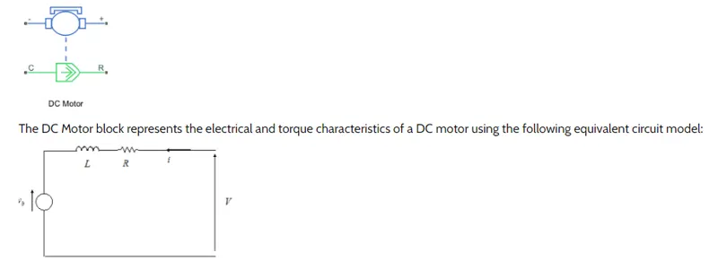
The resistor /7corresponds to the resistance you specify in the Armature resistance parameter. The inductor L corresponds to the inductance you specify in the Armature inductance parameter. DC motor block is used to supply propulsion power to the wheel through the gearbox. There are various types of DC motor block such as BLDC, PMDC, etc based on the propulsion requirement proper motor is used as per the voltage supply conditions.
Electrical ports:
• -: Negative terminal
• +: Positive terminal
Mechanical ports:
• R - Motor rotor
• C - Motor case
As DC motor block contains two parts one is electrical and another is mechanical. The electrical part is connected to the controller port and the machine is connected to the gearbox and electrical reference. The parameters of the DC motor can be changed as per the required conditions. Here we have chosen as rated power and no-load speed.
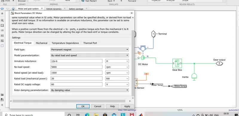
As the rated power in an electric vehicle is in kW so we change W to kW and it is a range of 50-100 we have kept here as 50 kW of rated power. According to vehicle speed and gear ratio rated speed can be changed here we have taken as 3000rpm as the rated speed of the motor and no-load speed as 5000 rpm.
The battery pack contains various cells of 3.6kW of power each and are connected in series and parallel combination for supplying the power supply voltage as per the rated power. Here we have taken the rated DC supply voltage as 80 V.
H-Bridge:-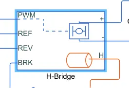
Description
The H-Bridge block represents an H-bridge motor driver. The block has the following two Simulation mode options:
PWM — The H-Bridge block output is a controlled voltage that depends on the input signal at the PWM port. If the input signal has a value greater than the Enable threshold voltage parameter value, the H-Bridge block output is on and has a value equal to the value of the Output voltage amplitude parameter. If it has a value less than the Enable threshold voltage parameter value, the block maintains the load circuit using one of the following three Freewheeling mode options:
Via one semiconductor switch and one freewheeling diode
Via two freewheeling diodes
Via two semiconductor switches and one freewheeling diode
The first and third options are sometimes referred to as synchronous operation.
The signal at the REV port determines the polarity of the output. If the value of the signal at the REV port is less than the value of the Reverse threshold voltage parameter, the output has positive polarity; otherwise, it has negative polarity.
Averaged — This mode has two Load current characteristics options:
Smoothed
Unsmoothed or discontinuous
The Smoothed option assumes that the current is practically continuous due to load inductance. In this case, the H-Bridge block output is:
VO
VPWM
APWM
−IOUT
RON
where:
VO is the value of the Output voltage amplitude parameter.
VPWM is the value of the voltage at the PWM port.
APWM is the value of the PWM signal amplitude parameter.
IOUT is the value of the output current.
RON is the Bridge on resistance parameter.
The current will be smooth if the PWM frequency is large enough. Synchronous operation where freewheeling is via a bridge arm back to the supply also helps smooth the current. For cases where the current is not smooth, or possibly discontinuous (that is, it goes to zero between PWM cycles), use the Unsmoothed or discontinuous option. For this option, you must also provide values for the Total load series resistance, Total load series inductance, and PWM frequency. During simulation, the block uses these values to calculate a more accurate value for H-bridge output voltage that achieves the same average current as would be present if simulating in PWM mode.
Set the Simulation mode parameter to Averaged to speed up simulations when driving the H-Bridge block with a Controlled PWM Voltage block. You must also set the Simulation mode parameter of the Controlled PWM Voltage block to Averaged mode. This applies the average of the demanded PWM voltage to the motor. The accuracy of the Averaged mode simulation results relies on the validity of your assumption about the load current. If you specify that the current is Unsmoothed or discontinuous, then the accuracy also depends on the values you provide for load resistance and inductance being representative. This mode also makes some simplifying assumptions about the underlying equations for the case when current is discontinuous. For typical motor and bridge parameters, accuracy should be within a few percent. To verify Averaged mode accuracy, run the simulation using the PWM mode and compare the results to those obtained from using the Averaged mode.
Braking mode is invoked when the voltage presented at the BRK port is larger than the Braking threshold voltage. Regardless of whether in PWM or Averaged mode, when in braking mode the H-bridge is modeled by a series combination of two resistances R1 and R2 where:
R1 is the resistance of a single bridge arm, that is, half the value of the Total bridge on resistance parameter.
R2 is the resistance of a single bridge arm in parallel with a diode resistance, that is, R1 · Rd / ( R1 + Rd ), where Rd is the diode resistance.
PID Controller:-
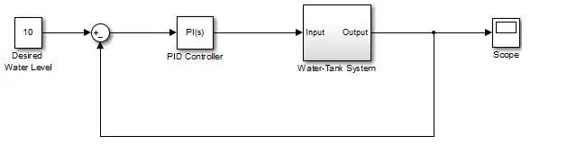
Description
The PID Controller block implements a PID controller (PID, PI, PD, P only, or I only). The block is identical to the Discrete PID Controller block with the Time domain parameter set to Continuous-time.
The block output is a weighted sum of the input signal, the integral of the input signal, and the derivative of the input signal. The weights are the proportional, integral, and derivative gain parameters. A first-order pole filters the derivative action.
The block supports several controller types and structures. Configurable options in the block include:
Controller type (PID, PI, PD, P only, or I only) — See the Controller parameter.
Controller form (Parallel or Ideal) — See the Form parameter.
Time domain (continuous or discrete) — See the Time domain parameter.
Initial conditions and reset trigger — See the Source and External reset parameters.
Output saturation limits and built-in anti-windup mechanism — See the Limit output parameter.
Signal tracking for bumpless control transfer and multiloop control — See the Enable tracking mode parameter.
As you change these options, the internal structure of the block changes by activating different variant subsystems. (See Variant Subsystems.) To examine the internal structure of the block and its variant subsystems, right-click the block and select Mask > Look Under Mask.
Battery:-
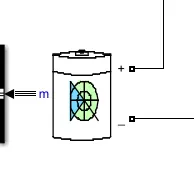
The Battery block implements a generic dynamic model that represents most popular types of rechargeable batteries.
This figure shows the equivalent circuit that the block models.
Charge and Discharge Characteristics
The circuit parameters can be modified to represent a specific battery type and its discharge characteristics. A typical discharge curve consists of three sections.
The first section represents the exponential voltage drop when the battery is charged. The width of the drop depends on the battery type. The second section represents the charge that can be extracted from the battery until the voltage drops below the battery nominal voltage. Finally, the third section represents the total discharge of the battery, when the voltage drops rapidly.
When the battery current is negative, the battery recharges, following a charge characteristic.
The model parameters are derived from the discharge characteristics. The discharging and charging characteristics are assumed to be the same.
The Exp(s) transfer function represents the hysteresis phenomenon for the lead-acid, nickel-cadmium (NiCD), and nickel-metal hydride (NiMH) batteries during the charge and discharge cycles. The exponential voltage increases when a battery is charging, regardless of the battery's state of charge. When the battery is discharging, the exponential voltage decreases immediately.
The state of charge (SOC) for a battery is a measure of battery's charge, expressed as a percent of the full charge. The depth of discharge (DOD) is the numerical compliment of the SOC, such that DOD = 100% - SOC.
For example, if the SOC is:
100% — The battery is fully charged and the DOD is 0%.
75% — The battery is 3/4 charged and the DOD is 25%.
50% — The battery is 1/2 charged and the DOD is 50%.
0% — The battery is has 0 charge and the DOD is 100%
Controlled Current Source:-
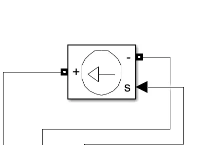
The Controlled Current Source block converts the Simulink® input signal into an equivalent current source. The generated current is driven by the input signal of the block. The positive current direction is as shown by the arrow in the block icon.
You can initialize the Controlled Current Source block with a specific AC or DC current. If you want to start the simulation in steady state, the block input must be connected to a signal starting as a sinusoidal or DC waveform corresponding to the initial values.
Note
The Simulink input signal must be a complex value (phasor) when you are using the Controlled Current Source block in a phasor simulation, because in this case, Simscape™ Electrical™ Specialized Power Systems software does not automatically convert the input signal from time-domain into complex (phasor) signal.
Parameters
Initialize
Default is selected. If selected, initializes the Controlled Current Source block with the specified Initial current, Initial phase, and Initial frequency parameters.
Source type
The Source type parameter is not visible if the Initialize parameter is not selected.
The type of current source. Select AC (default) to initialize the Controlled Current Source Block as an AC current source. Select DC to initialize the Controlled Current Source block as a DC current.
Initial amplitude
This parameter is not visible in the dialog box if the Initialize parameter is cleared. The initial peak current for the initialization of the source, in amperes (A). Default is 0.
Initial phase
The initial phase for the initialization of the source, in degrees. Default is 0. The Initial phase parameter is not visible in the dialog box if the Source type parameter is set to DC.
Initial frequency
The initial frequency for the initialization of the source, in hertz (Hz). Default is 0. The Initial frequency parameter is not visible in the dialog box if the Source type parameter is set to DC.
Measurements
Default is None. Select Current to measure the current flowing through the Controlled Current Source block.
Place a Multimeter block in your model to display the selected measurements during the simulation. In the Available Measurements list box of the Multimeter block, the measurement is identified by a label followed by the block name:
Vehicle model Subsystems:
1. Transmission system.
Explanation:
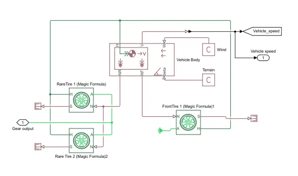
• As we know transmission is the main part of the vehicle which is used to supply the propulsion powers from the motor and the battery to the wheels. • Under transmission, the number of components comes which are wheels, gearbox, throttle, power input etc.
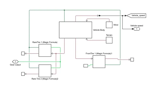
• In this transmission subsystem blocks used are Tire and vehicle body.
• There are 3 tire blocks used as 3 wheels of the rickshaw and here we have connected the gearbox with the rear wheel to make it a rear-wheel drive.
• The vehicle body block is been connected to these wheels by all the input and output ports.
• In-vehicle body block we have connected as ps constant block to beta and wind velocity as we have assumed both as zero and hub motor port is also connected with the wheels H port.
2. DC Motor system.
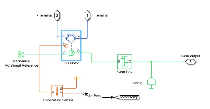
Mechanical Rotational Reference
Temperature Sensor
Explanation:
• Here we used a DC motor as a power source to the gearbox.
• Here also we have enabled the thermal port to get the temperature output while the motor is running to give power supply to the gearbox.
• Here we have used inertia block to give the initial start in a positive direction to the shaft which is connected between motor and gearbox.
3. Motor controller.
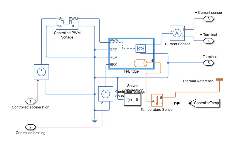
Explanation:
• This motor controller subsystem contains H-Bridge and a Controlled PWM Voltage block.
• H-Bridge block is used to supply the power from the battery to the DC motor.
• H-Bridge has 4 switches that give the controlled DC voltage supply to the DC motor and we can also control the supply of voltages.
• Here we have enabled the thermal output of the H-bridge controller to get the temperature output of the controller while the vehicle is in motion.
• In H-Bridge we have control on PWM voltage, Reverse and braking effect also.
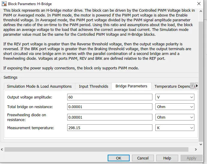
• As below we can see block parameters, for simulation mode we have two options internal and external as we choose internally we have a choice of PWM mode and averaged mode.
• In PWM mode the simulation time increases drastically as if the simulation time is of 5 secs then PWM mode is effective but as now our simulation time is in mins or hours so here averaged mode is been chosen as it is faster compared to PWM mode.
• Also, we have kept regenerative mode enable and load current characteristics as smoothed.
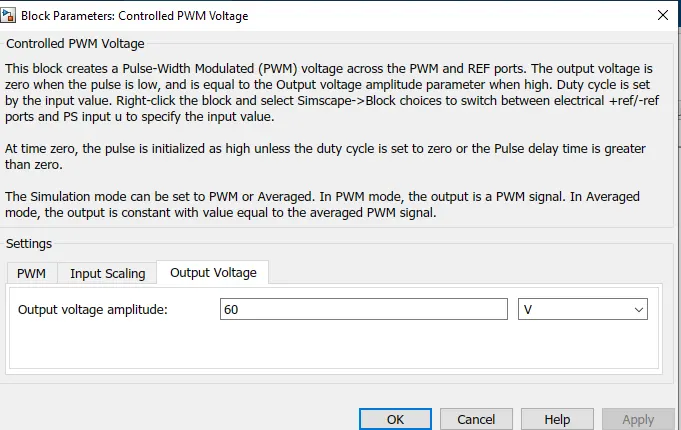
• Also, we have to change the output voltage amplitude to the voltage we have supplied to the DC motor.
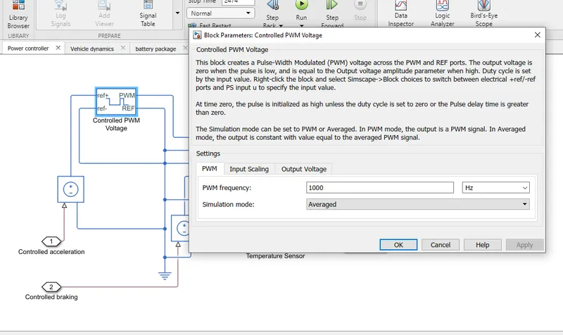
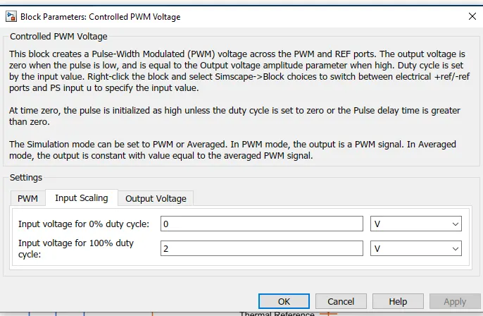
• As from the Controlled PWM voltage block which is connected to the input PWM Pin in the H-Bridge block.
• This block will apply pulses and based on these pulses from the fixed battery voltage variable output voltage will be available to the motor and the motor speed and motor torque are changed.
• So basically this subsystem will control the power supply to the DC motor using the following blocks.
3.SOC calculation. 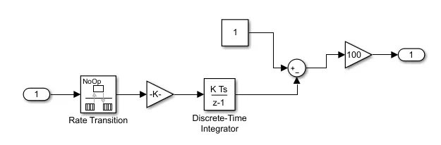
Explanation:
• Here in this subsystem, there is the number of blocks used are rate transition, gain, constant, add, etc.
• Rate transition block takes input from the controlled current source block as soc input signals and do a sampling of the signals and gives to gain block.
• Gain block multiplies the sampling signal with the rated voltage and gives it to the discrete-time integrator block.
• Discrete-time integrator block integrates the signal and adds it to the constant given and supply is to the gain block again.
• Gain block multiplies it with the 100 and gives it to the SOC output.
4. Battery pack system.
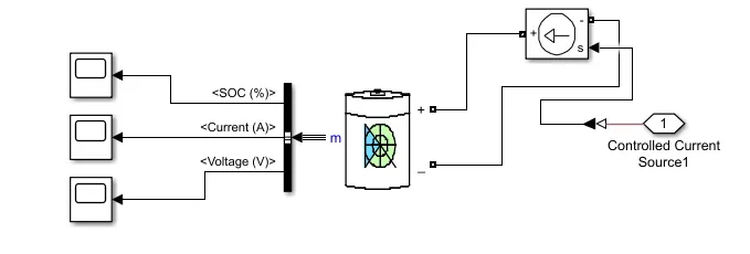
Explanation:
• Here we have used a lithium-ion battery block to give the current and voltage supply to the rickshaw.
• A controlled current source block is used so that there is no excessive load on the battery if there is a change in speed or torque value.
• We have a bus selector block that takes the battery performance and gives us its SOC state, Current discharge and voltage supplied by the battery.
Case-I: For FTP75 drive cycle:
Input model:
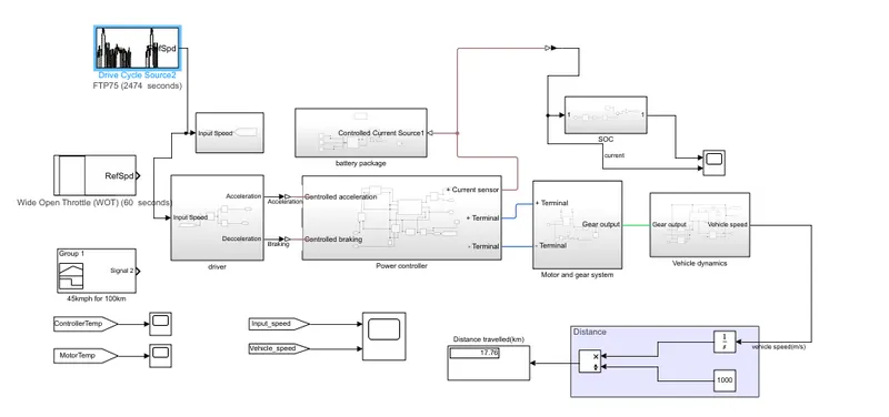
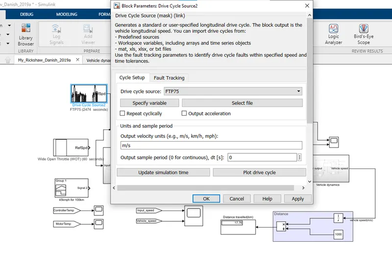
Input parameters:
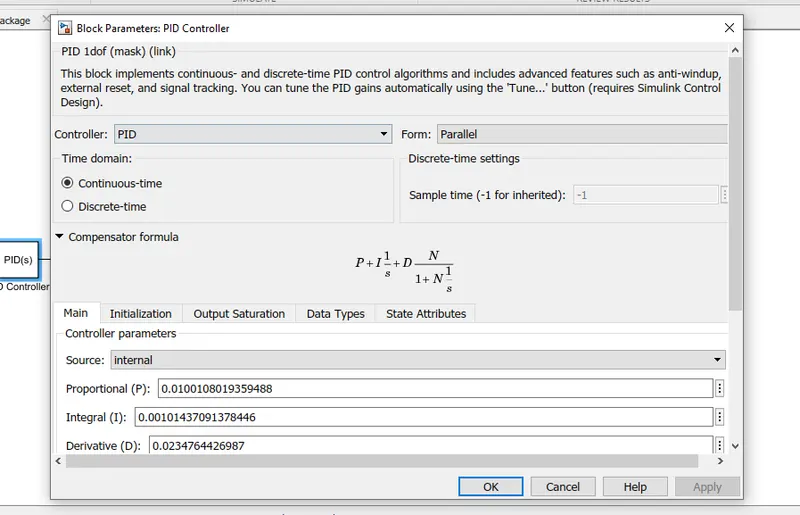
1- PID block parameters
2- DC Motor:
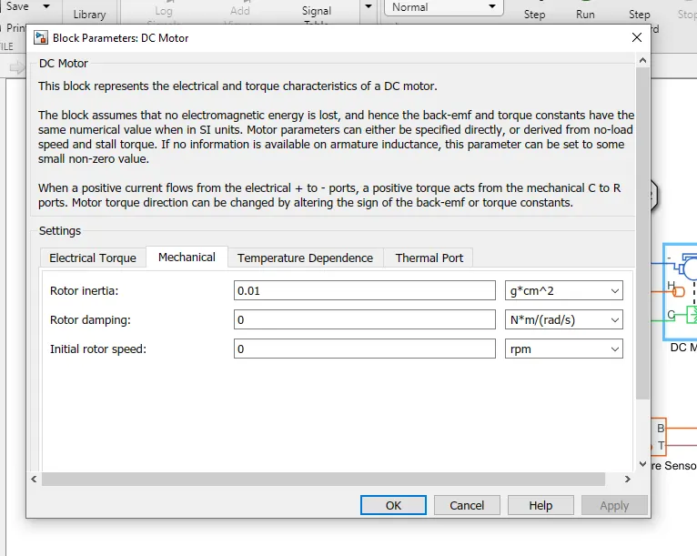
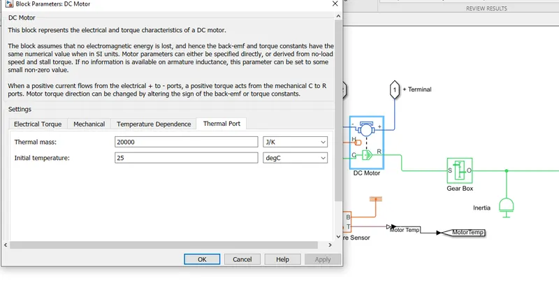
3)H-Bridge
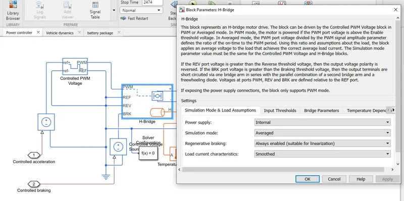
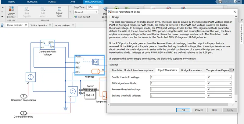
4- Controlled PWM voltage block:
Output: 1- Distance travelled: 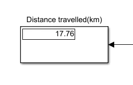
• Distance travelled by the vehicle is 17.76km for the applied voltage of 60V. • This distance is calculated using velocity feedback given.
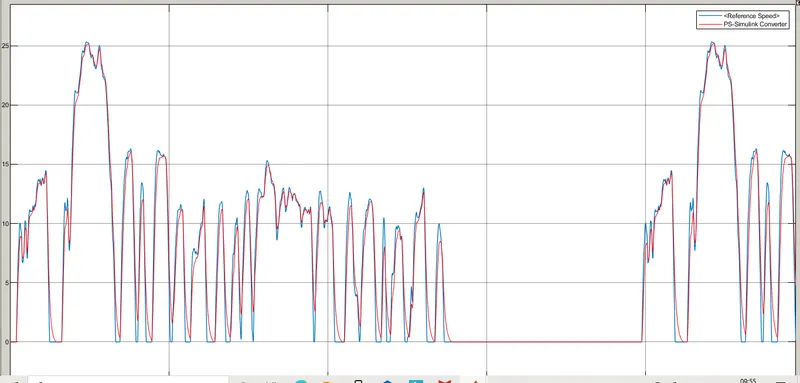
2- Velocity:
Result:
• Here the input given to the vehicle velocity was the FTP75 drive cycle.
• Here we can observe that velocity by the vehicle is approximately the same as of standard drive cycle given as input.
• As here we can observe while steep braking of the vehicle, our vehicle takes more time for the braking as the standard drive cycle.
• While acceleration also vehicle takes comparatively more time to get at that peak velocity. • As per the standard drive cycle peak velocity attained by the vehicle is 25m/s but the velocity traced by the vehicle is about 23-24m/s which is almost similar.
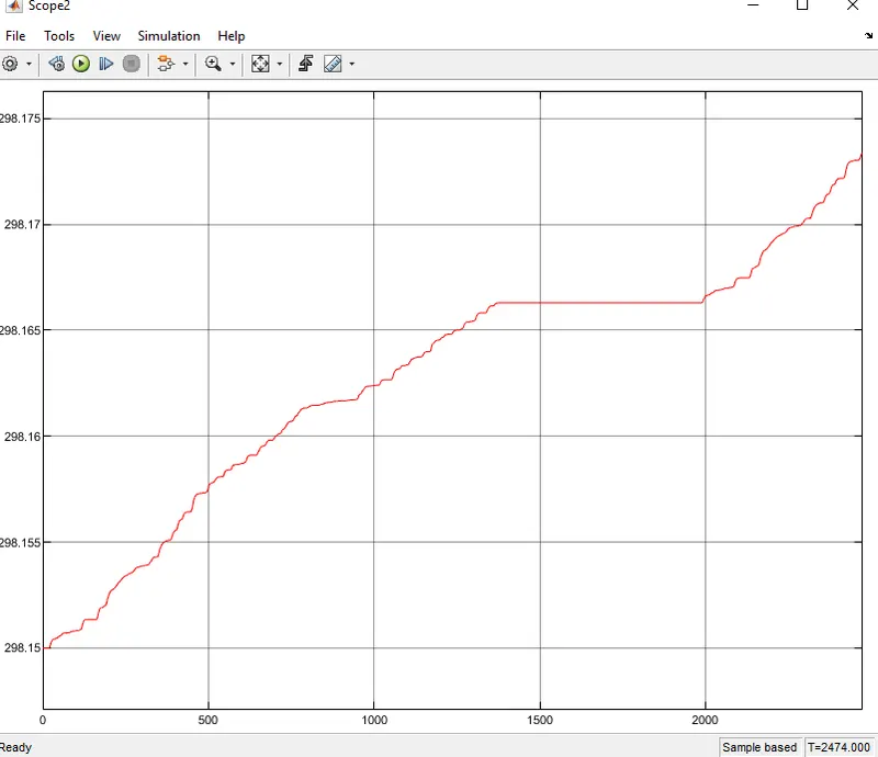
3- Temperature output of Motor controller(H-Bridge):
Result:
• Here as per the drive cycle as speed increase the temperature also increases and as hen vehicle deaccelerates temperature all decreases.
• From 1400sec to 2100 sec we can observe there is a constant path which means there is no change in temperature.
• The initial temperature of the controller was 298.15 and the final temperature after completing the drive cycle was 298.17.
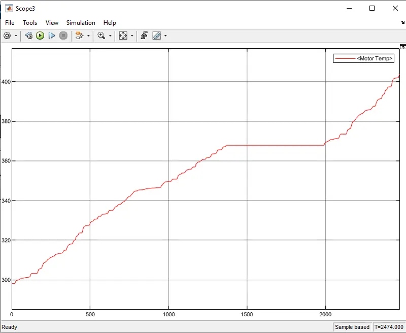
4- DC motor temperature output:
Result:
• Here as per the drive cycle as speed increase the temperature also increases and as hen vehicle deaccelerates temperature all decreases.
• From 1400sec to 2100 sec we can observe there is a constant path which means there is no change in temperature.
• The initial temperature of the controller was 298 and the final temperature after completing the drive cycle was 385.
• The temperature rise is more as compared to the controller temperature.
5- SOC:
Result:
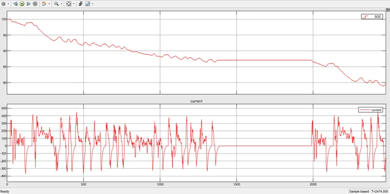
• Here we gave the input as FTP75 drive cycle and run the model for 2474 sec.
• So here we can observe the SOC of the battery is been discharged by 1.5% of the total 100% battery charge.
• SOC of the battery is 99.2% after the drive cycle is completed.
• As we observe the graph there is no steady-state in the signal sometimes it is going up and sometimes its going down, while the curve is going down means the battery is getting discharged and while the curve is going up it means the battery is getting charged again.
• The battery is getting charged due to regenerative braking.
• The maximum discharge SOC of the battery is 98.5.
• From 1200sec to 2000 sec the battery is discharging continuously.
Case-2: For WOT drive cycle:
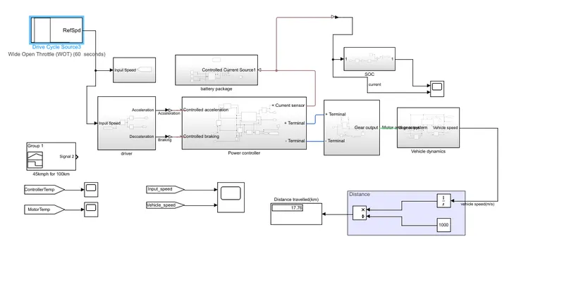
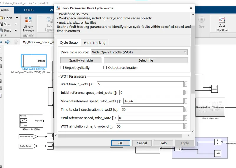
Input parameters: 1-Drive cycle(WOT)
Output: 1- Distance travelled: 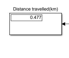
Disctance covered
0.477
Result:
• Distance travelled by the vehicle is 0.477km for the applied voltage of 60V. • This distance is calculated using velocity feedback given.
2- Velocity:
2- Velocity:
Result:
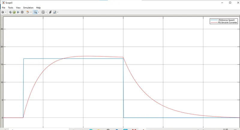
• Here for WOT, the output which we are getting is almost similar to the value which we gave to the block parameters.
• While acceleration signal is getting exponentially increased and it is taking almost 18 sec to achieve 45kmph or 16.66m/s of speed which we gave as the WOT input condition.
• Also while deacceleration the vehicle takes more time to come at rest. It almost takes 12sec to deaccelerate the vehicle to 0.
3- DC motor temperature output:
Result:
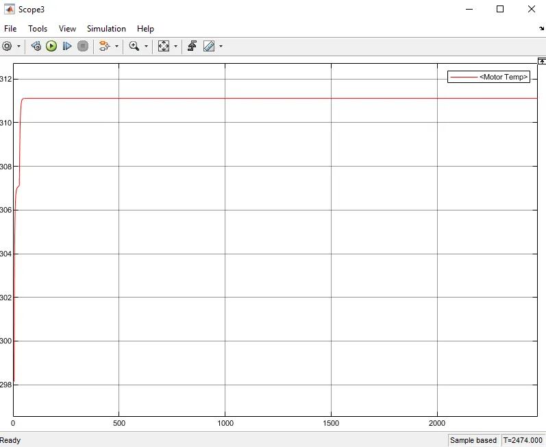
• Here as we can observe temperature rise when the vehicles accelerated and it is constant when the vehicle speed is constant.
• If we compare it with WOT drive cycle we can observe that while deceleration also there is a rise in temp this is due to regenerative braking effect as the motor act as a generator at that time and it charges the battery and the controller are controlling the generator parameters.
• The maximum temperature attends by the motor is 305.5.
4- Temperature output of Motor controller(H-Bridge):
Result:
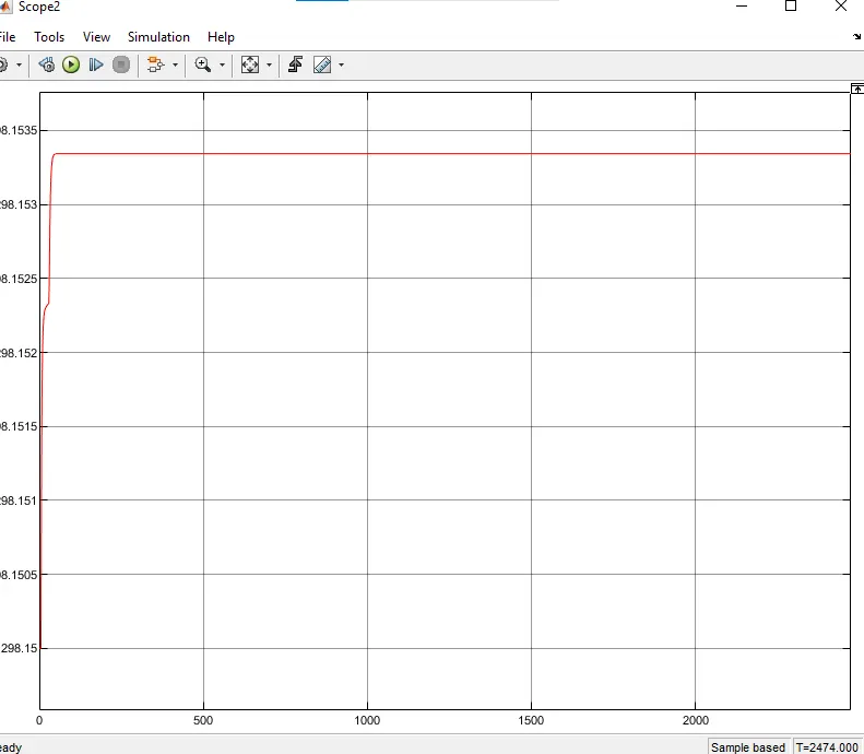
• Here as we can observe temperature rise when the vehicles accelerated and it is constant when the vehicle speed is constant.
• If we compare it with WOT drive cycle we can observe that while deceleration also there is a rise in temp this is due to regenerative braking effect as the motor act as a generator at that time and it charges the battery and the controller are controlling the generator parameters.
• The maximum temperature attend by the controller here is 298.152.
5-SOC:
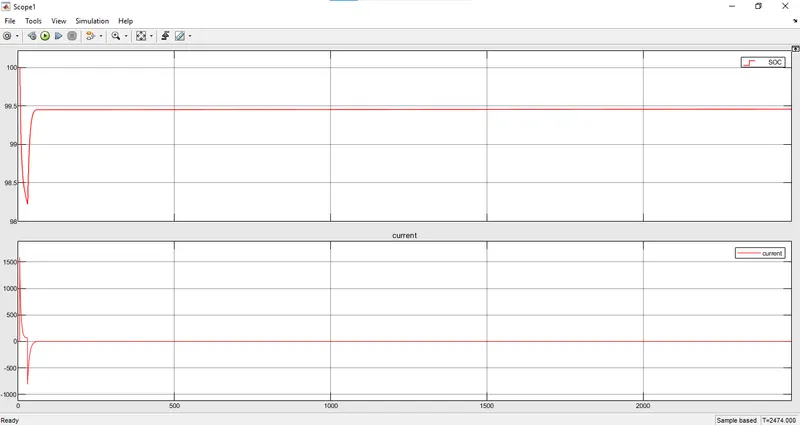
Result: • Here for the WOT drive cycle, the output for SOC we arc getting is the battery is discharged by 0.2% out of 100% of the total charge.
Case-3: For 40 kmph constant speed up to 100 km using signal builder block:
Input model:
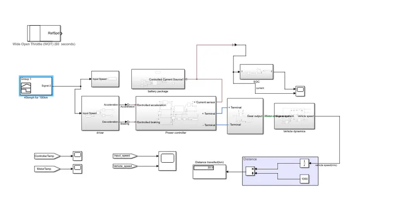
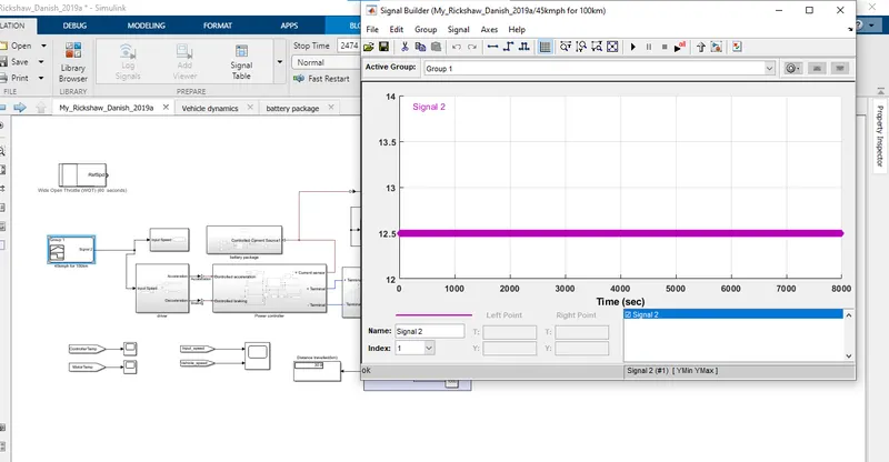
Output:
1-Distance travelled:
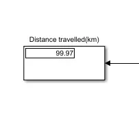
Disctance covered
99.961
Result: • Distance travelled by the vehicle is 99.96km for the applied voltage of 60V.
• This distance is calculated using velocity feedback given.
2- Velocity:
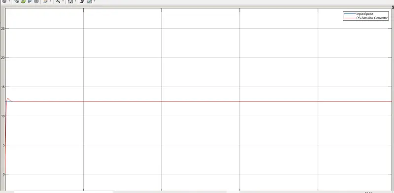
Result
• Here we can observe that as per the input value output is 100% accurate and we are achieving the 45kmph of constant speed for 100km of range.
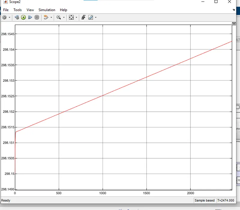
3- Temperature output of Motor controller(H-Bridge):
Result:
• We can observe here is that as for the constant speed the temperature of the controller increases linearly. • The maximum temperature of the controller attained is 298.151.
• As the distance travelled increases temperature of the controller increases.
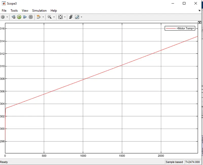
4- DC motor temperature output
Result:
• We can observe here is that as for the constant speed the temperature of the DC motor increases linearly.
• The maximum temperature of the DC motor attained is 315.
• As the distance travelled increases temperature of the DC motor increases.
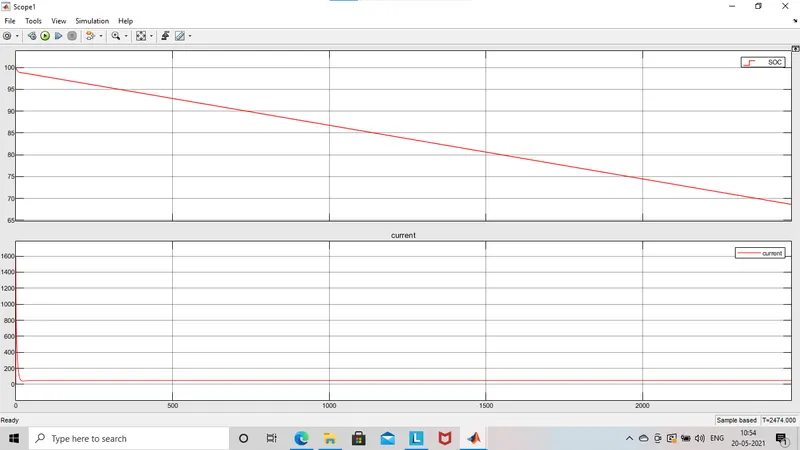
5- SOC:
Result:
• Here we can observe the SOC of the battery is decrease throughout the 100 km range.
• SOC is 65% after the 100km of range.
Conclusion:
• We successfully modelled and simulated the Electric Rickshaw.
• Results are been plotted for the temperature of controller, energy consumption, the temperature of DC motor and also 100km range at a constant speed of 45 kmph.