Final Project: Electric Rickshaw modelling

AIM :  Design of an Electric Rickshaw using MATLAB Simulink.

ABSTRACT :

In this project, we going to build the MATLAB model of the ELECTRIC RICKHAEW by using a PM brushed type DC motor and a suitable Lithium-Ion battery for the motor. Before that, we will know about what is Electric RICKHAEW, how it's works and the benefits of EV RICKHAE. Then we make an actual EV RICKHAEW model in SIMULINK with suitable blocks from the powertrain block set. My main motto is to check "how my RICKHAEW performs for any three standard driving cycles showing energy consumption, the temperature rise of motor and controller for vehicle cover around 100 km at constant speed driving 45 kmph. Made a comparison with Mahindra e-Rickhaew and my Simulink model.

INTRODUCTION

Electric E-Rickshaw is also known as electric tuk-tuk, e-rickshaw and auto which are going more popular after 2018 in Indian market. This E-rickshaw is best alternative of petrol/ CNG auto rickshaw and human or horse pulled rickshaws because of their low fuel cost, zero emissions and less human efforts.

The electrical system used in Indian version is 48VDC can run 90– 100 km/full charge, top speed 25 km/hour and this electric motor power ranging from 650-1400 Watts; the battery takes 8–10 hrs to become fully charged. Basic seating capacity is driver plus 4 passenger total 5 persons.

Here basically, e-rickshaw is designed in CREO and MATLAB Simulink. In the designed electric rickshaw main blocks are battery, drive cycle, controlled, DC Motor, Vehicle body and transmission system. Drive cycle is the input of human effort that how he is going to drive his actual cycle. We can use drive cycle like FTP75, WOT or by using Excel.

The main objective of this project is to obtain speed by driver, to estimate the temperature of motor and controller, to estimate the state of charge (SOC) and distance travel by the vehicle. There is a SOC block that will estimate the state of charge of battery, distance is calculated by speed and time parameter for all the three Drive cycle.

The electric vehicle consists of a battery, motors, and controller then it generates propulsion power.To design any vehicle 1st we have to calculate propulsion power, then the motor is selected.Lastly based on the motor rating or operating range and no km/charge we want to depend on everything battery capacity and then battery capacity is selected. So the Design flow of vehicle engineer has to be like the following.Identify what amount of propulsion power required.What is the best suitable motor for that propulsion power.Then type of battery and range of battery according to the range.

Design and Construction :

• These rickshaws have an M.S(Mild Steel) tubular chassis, consisting of three wheels with a differential mechanism at the rear wheels. The motor is a brushless DC motor manufactured mostly in India and China. The electrical system used in the Indian version is 48V and in Bangladesh is 60V. The body design from the most popular Chinese version is of very thin iron or aluminum sheets. Vehicles made in fiber are also popular because of their strength and durability, resulting in low maintenance, especially in India.
• The body design is varied from load carriers, passenger vehicles with no roof, to full body with windshield for drivers comfort. It consists of a controller unit. They are sold on the basis of voltage supplied and current output, also the number of MOSFET (metal oxide field-effect transistors) used. The battery used is mostly a lead-acid battery with life of 6–12
  months. Deep cycle batteries designed for electric vehicles are rarely used. The weight of the electric car has also been a recurring design difficulty in them.

General detail of E-Rickshaw

• Battery Type Lithium Ion 60.8 V 160 Ah
• Vehicle kerb weight 260 kgs
• Load capacity 340 kgs
• Vehicle speed 7 kmph
• Driving range 140 km (160 Ah)
• No of wheels per axel 2
• Frontal Area 91m²
• Drag coefficient 5
• Wheel radius 306m
• Vertical load 3000 N
• Nominal Voltage 8 V
• Rated Capacity 160 Ah
• Initial SOC % 100
• Internal Resistance 5 ohm

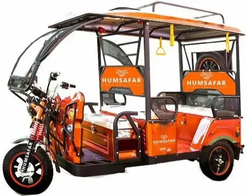
A CAD model of Electric rickshaw is shown below.

• Electric Motor: PM brushed DC Motor type 650- 1400W & 48V (Input) motor is used. It is controlled via an electronic controller.
• Electronic Motor Controller: The controller includes a manual or automatic switch turning the motor on/off, selecting forward or reverse motion, selecting and regulating speed, regulating or limiting torque and protecting against overloads. It is connected to battery pack and controller feeds the input to the motor, lamp, AC/DC converter and Speedometer/ Indicator.
• Battery: Set of four 12V deep cycles /Li-ion batteries are used since the required voltage is 48V. These batteries are connected in series to the controller unit.
• Front Shock Absorbers: Helical Spring with dampener with hydraulic telescopic shock absorbers are used.
• Rear Suspension: Leaf spring carriage spring with rear shocker
• Brakes: Drum brakes, actuated internally, expanding shoe type are used. Brakes are mounted on the chassis (Pedal brakes), so on pressing the pedal, the brakes will engage stopping the rear wheels.
• Speedometer/Indicator: Speedometer generally used have analogue dials. The one the left side indicates vehicle speed and one on the right side indicate battery charge level. It is connected to the controller unit.
• Steering: Handle bar type steering is used.
• Miscellaneous Spare parts: Centre locking, Alloy wheel, Rear light, Front glass, Front Indicator, Headlight, Ignition switch, Charger, Converter, left-right switch, Tyre, Wirings, Throttle set etc.

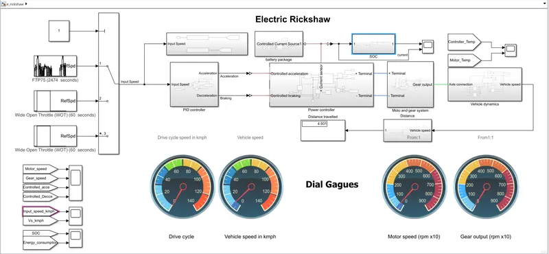
As we can see that the above diagram is consisting of MATLAB Simulink model of an electric rickshaw. In above model we use three type of different drive cycle to run the vehicle body. A basic current is applied to the model. The required voltage to the vehicle is controlled by the controller. Depending upon the vehicle parameter the controller will follow the drive cycle and run the motor.

Battery :

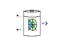
• The battery is required to power the controller and motor. The controller uses the battery power according to produce the input given by the motor to obtain maximum speed. The battery is also used to power every electrical component in the vehicle.
• The Battery block implements a generic dynamic model that represents most popular types of rechargeable batteries.

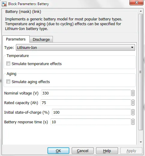
• The battery has two stage one is charging and another one is discharging state. The battery is of 75Ah capacity.
  The Nominal voltage of battery is 330 V
  Initial SoC is of 100%
  The battery as a series internal resistance plus a charge-dependent voltage source defined by :
  V=Vnom⋅SoC1-β⋅(1-SoC)">V=Vnom⋅SoC1−β⋅(1−SoC)�=����⋅���1-�⋅(1-���)
• where SoC is the state of charge and Vnom is the nominal voltage. Coefficient beta is calculated to satisfy a user-defined data point [AH1,V1].
• The battery has a positive and negative terminal which is given the voltage-controlled source where the battery consumption is controlled by the motor controller and then it is given to the SOC block.

Full Model Parameter

Drive cycle

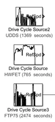
Here I have used three different type of drive cycle which are as given below.

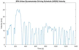
UDDS Drive Cycle

Urban Dynamometer Driving Schedule

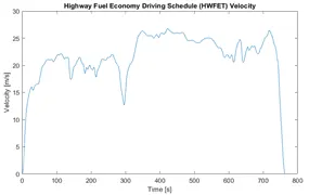
HWFET Drive Cycle

Highway Fuel Economy Driving Schedule

FTP Drive cycle

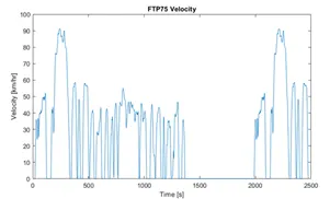
Generate a standard or user specified longitudinal drive cycle.

Battery State of Charge :

• SoC is the percentage or level of battery presents after certain travel or consumption of battery charge by the vehicle.
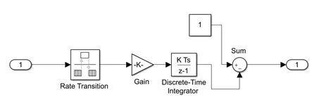
• In the designed vehicle battery charge or SOC is calculated by the giving it to the rate transition and then to gain where 1/(nominal battery capacity) then to a discrete-time integrator and it will get minus from the 1 as it is considered a 100% of battery and it is multiplied with 100 to get percentage of battery.
• The majority of blocks are simscape blocks where physical to simulink converter is used to convert the physical signal from simscape block to simulink signal.

Controlled Current Source :

The Controlled Current Source block converts the Simulink input signal into an equivalent current source. The generated current is driven by the input signal of the block. The positive current direction is as shown by the arrow in the block icon.

We can initialize the Controlled Current Source block with a specific AC or DC current. If we want to start the simulation in steady state, the block input must be connected to a signal starting as a sinusoidal or DC waveform corresponding to the initial values.

• Double click controlled current source and from drop down menu of measurement select current.
• Signal output will connect with scope by adding current signal to it.
• (+) terminal will connect with battery (-) terminal.

BUS Selector :

The Bus Selector block outputs the signals you select from the input bus. The block can output the selected elements separately or in a new virtual bus.

• Here just we have mange the output and connect with different Scope Block.

PowerGUI :

The powergui block allows us to choose one of these methods to solve your circuit :

• Continuous, which uses a variable-step solver from Simulink
• Discretization of the electrical system for a solution at fixed time steps
• Continuous or discrete phasor solution

The powergui block also opens tools for steady-state and simulation results analysis and for advanced parameter design.

PROCEDURE :

(1) Vehicle Body Subsystem Model :

• Motor will produce the rotational output which will give to the vehicle body and transmission system. The rotational output is taken by the gear system here to maintain the constant speed throughout the transmission without any loss in speed from the motor to tires.
• Below is a diagram that is how it is how it inside the vehicle body and transmission system and in the main design, it is referred just only as a transmission system.
• Here I created a Rear wheel drive transmission system.

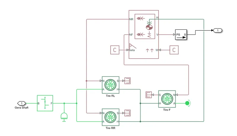
• The gear output is given to axels of Rear tires, in the circuit it is shown that gear is connected to Rear wheels and front tire is free to rotational motion, thus vehicle moves forward. N is the normal force caused by the tires and it is given to the vehicle body normal force port.
• The vehicle body has an H-Hub, S- Tire slip, N- Normal force, A- axel connection, wind velocity, inclination angle. The tires hub is connected as a common node to the vehicle body.
• The vehicle body wind velocity is connected to a constant block and the beta-inclination angle is connected to another constant block where we can assign wind velocity and inclination angle as per requirement. Velocity is the output port where we can get at which speed the vehicle is moving. The velocity is taken out to the get the distance travelled and state of charge.

Vehicle Body Parameters :

• Vehicle body mass, Centre of gravity distance values and aerodynamic drag variables are modified.
• Pitch dynamics are kept ON with other variable values as default values.

Tire :

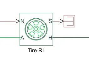
• Represents the longitudinal behavior of a highway tire characterized by the tire Magic Formula. The block is built from Tire-Road Interaction (Magic Formula) and Simscape Foundation Library Wheel and Axle blocks. Optionally, the effects of tire inertia, stiffness, and damping can be included.

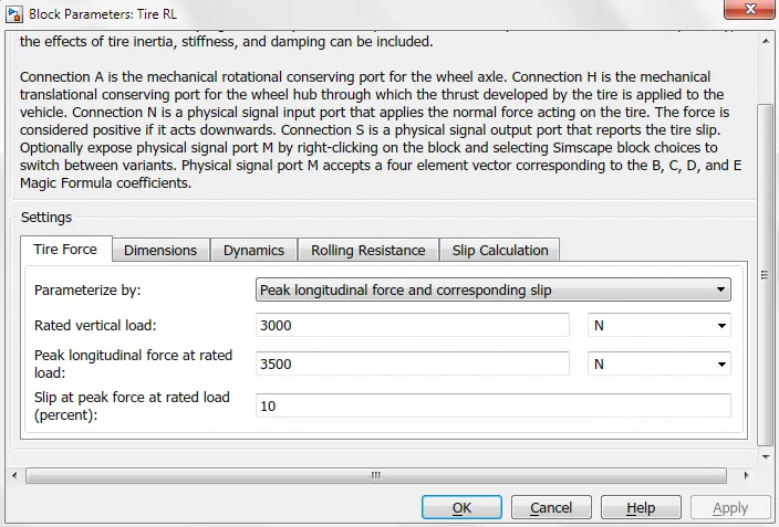
• Connection A is the mechanical rotational conserving port for the wheel axle. Connection H is the mechanical translational conserving port for the wheel hub through which the thrust developed by the tire is applied to the vehicle. Connection N is a physical signal input port that applies the normal force acting on the tire. The force is considered positive if it acts downwards.
• Connection S is a physical signal output port that reports the tire slip. Optionally expose physical signal port M by setting Parameterize by to Physical signal Magic Formula coefficients. Physical signal port M accepts a four element vector corresponding to the B, C, D, and E Magic Formula coefficients.

Gear :

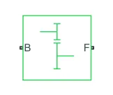
• Represents a fixed-ratio gear or gear box. No inertia or compliance is modeled in this block. You can optionally include gear
  meshing and viscous bearing losses.

MODELLING OF VEHICLE BODY SYSTEM:

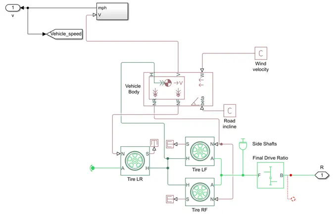
The above figure highlights the vehicle body for electric rickshaw which is having rear axle drive. The Vehicle Body block represents a two-axle vehicle body in longitudinal motion.

Longitudinal Driver :

• Longitudinal Driver is an inbuilt block provided by the powertrain blockset.

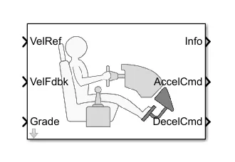
• It is a parametric longitudinal speed tracking controller for generating normalized Acceleration and Braking commands based on reference and feedback velocities.
• The VelFdbk port corresponds to the feedback velocity. The actual velocity output given by the vehicle body is connected here. By comparing the actual (feedback) velocity with the reference velocity, the driver block generates acceleration and braking signals in order to minimise the error between the two concerned velocities.
• Grade corresponds to the grade angle. For this simulation, no inclination is considered and hence, a constant block with value 1 is connected.
• Info gives the output for the bus signal for different block calculations like difference in reference vehicle speed and vehicle speed, etc.
• AccelCmd & DecelCmd correspond to the acceleration and deceleration commands generated respectively and are connected to the corresponding ports of the Controlled PWM Voltage block.
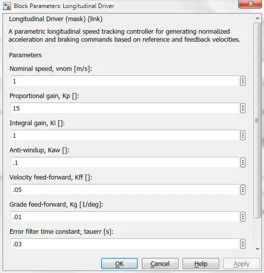
• Here, the selected control type is PI. Acordingly, the block implements proportional-integral (PI) control with tracking windup and feed-forward gains.

Controlled PWM Voltage :

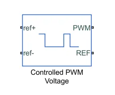
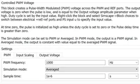
• This block creates a Pulse-Width Modulated (PWM) voltage across the PWM and REF ports. The output voltage is zero when the pulse is low, and is equal to the Output voltage amplitude parameter when high.
• Duty cycle is set by the input value. Right-click the block and select Simscape->Block choices to switch between electrical +ref/-ref ports and PS input u to specify the input value.
  
  
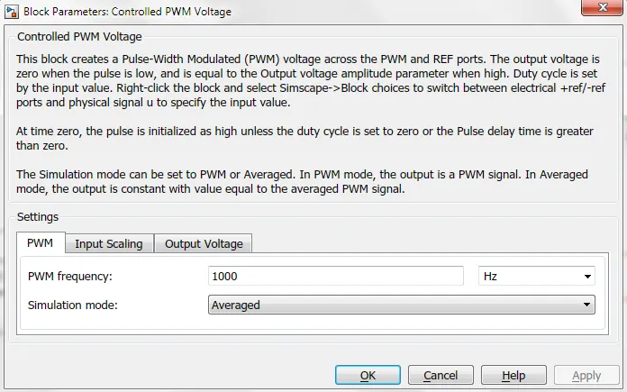
•  At time zero, the pulse is initialized as high unless the duty cycle is set to zero or the Pulse delay time is greater than zero.
• The Simulation mode can be set to PWM or Averaged. In PWM mode, the output is a PWM signal. In Averaged mode, the output is constant with value equal to the averaged PWM signal. Select Simulation mode as Averaged.

Temperature Sensor :

• Temperature Sensor is used to mesure the temperature of H-Bridge and Motor.

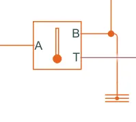
• This block measures temperature in a thermal network. There is no heat flow through the sensor. The physical signal port T reports the temperature difference across the sensor.
• The measurement is positive when the temperature at port A is greater than the temperature at port B.

Solver Configuration :

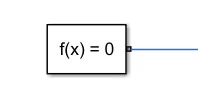
Defines solver settings to use for simulation.

SIMPLE GEAR

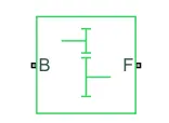
Simple Gear is a Final drive ratio which is a gearbox that constrains the connected driveline axes of the base gear and the follower gear.

B: The output B, base gear is connected with the input of DC motor R. It is a Rotational mechanical conserving port.

F: The output of F, follower gear is connected with the rear axle. It is also a Rotational mechanical conserving port.

In Simple Gear Block we can also do some changes according to our need.

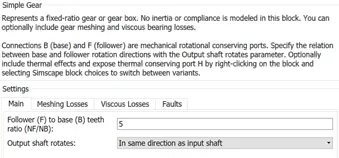
Main Setting

• Follower (F) to base (B) teeth ratio (NF/NB): 5, The value should be in Positive and it is a fixed ratio gFB of the follower gear to the base gear.
• Output shaft rotates: In the same direction as the input shaft, it is depending upon the direction of follower and base gear.

Meshing Losses

• Friction model: From drop-down, we can select Constant efficiency which calculates the Reduce torque transfer by a constant efficiency factor.
• Efficiency: 0.86, here we can change the efficiency depending upon our need, basically it is a Torque transfer efficiency between base gear shaft to the follower gear shaft.
• Follower power threshold: 0.001 W, it is an absolute value of the follower shaft power above which the full efficiency factor is in effect.

GOTO

GoTo block is used to display the vehicle speed.

CONFIGURATION BATTERY AND SOC

In given block there are some changes to configure the Lithium battery.

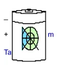
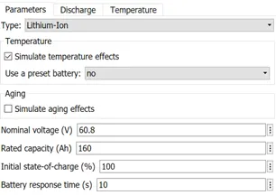
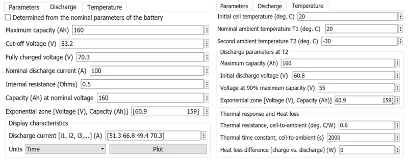
Basically, in battery a special change has done and i.e.

Under Parameter > Lithium-Ion (Change the following data)

• Nominal Voltage = 60.8 (V)
• Rated Capacity = 160 (Ah)

Under Discharge (Change the following data)

• Maximum Capacity = 160 (Ah)
• Cut-off Voltage = 53.2 (V)
• Fully Charged Voltage = 70.3 (V)
• Nominal Discharge Current = 100 (A)
• Internal Resistance = 0.5 (Ohms)
• Capacity at Nominal Voltage = 160 (Ah)

So, at Discharge rate of [51.3 66.8 49.4 70.3] the plot will be

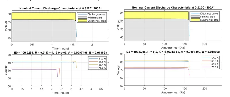
The circuit parameters can be modified to represent a specific battery type and its discharge characteristics. A typical discharge curve consists of three sections.

A basic block configuration and steps involve during whole system analysis.

Block used:

• PowerGUI
• Controlled Current Source
• Battery
• Temperature Ambient (Constant)
• Bus Selector
• Integrator
• Divide
• Product
• Time
• Scope

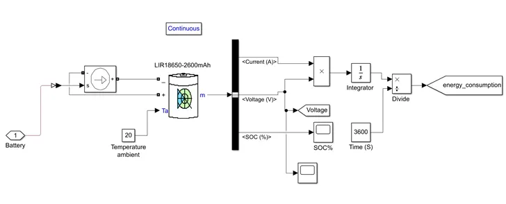
Controlled Current Source

The Controlled Current Source block converts the Simulink input signal into an equivalent current source. The generated current is driven by the input signal of the block. The positive current direction is as shown by the arrow in the block icon.

We can initialize the Controlled Current Source block with a specific AC or DC current. If we want to start the simulation in steady state, the block input must be connected to a signal starting as a sinusoidal or DC waveform corresponding to the initial values.

• Double click controlled current source and from drop down menu of measurement select current.
• Signal output will connect with scope by adding current signal to it.
• (+) terminal will connect with battery (-) terminal.

Battery

The Battery block implements a generic dynamic model that represents most popular types of rechargeable batteries.

• In battery setup just do the above changes which I highlighted above.
• Just connect ambient temperature with Ta input of battery.
• “M” will be connected with BUS selector lock.

BUS Selector

The Bus Selector block outputs the signals you select from the input bus. The block can output the selected elements separately or in a new virtual bus.

• Here just we have mange the output and connect with different Scope Block.

PowerGUI

The powergui block allows us to choose one of these methods to solve your circuit:

• Continuous, which uses a variable-step solver from Simulink
• Discretization of the electrical system for a solution at fixed time steps
• Continuous or discrete phasor solution

The powergui block also opens tools for steady-state and simulation results analysis and for advanced parameter design.

For calculating the SOC (State of Charge) we have to create a subsystem which will consist of Rate transition, Gain, Discrete Time Integrator, Constant and Sum blocks.

RATE TRANSITION

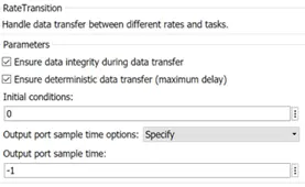
It is used to transfers data from the output of a block operating at one rate to the input of a block operating at a different rate.

Input Signal: Input signal to transition to a new sample rate, specified as a scalar, vector, matrix, or N-D array.

Output Signal: Output signal is the input signal converted to the sample rate you specify.

A basic input for this block is as

GAIN BLOCK

The Gain block multiplies the input by a constant value (gain). The input and the gain can each be a scalar, vector, or matrix.

Here Gain value is the multiplication element and the input is 1/(50×3600), where 50is battery ampere and 3600 is second.

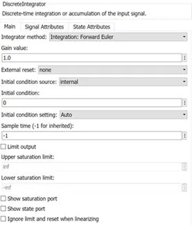
DISCRETE-TIME INTEGRATOR

The discrete-time integrator block is used for

• Define initial conditions on the block dialogue box or as input to the block
• Define an input gain (K) value
• Output the block state
• Define upper and lower limits on the integral
• Reset the state with an additional reset input

SUM BLOCK

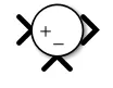
The Sum block performs addition or subtraction on its inputs.

In this block, the negative terminal will be connected with discrete-time integrator and positive terminal with constant.

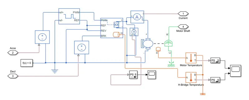
DC MOTOR WITH TEMPERATURE CALCULATION

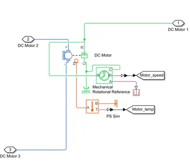
The DC Motor block represents the electrical and torque characteristics of a DC motor using the following equivalent circuit model:

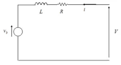
Here in this system, the positive terminal is connected with the current sensor negative terminal and negative terminal is connected with the negative terminal of H-Bridge.

R is DC motor rotor which connected with mechanical rotational port i.e. simple gear whereas C is DC motor case and it is connected with mechanical rotational reference.

A basic configuration of the DC motor is as follow:

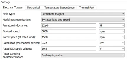
Here for the particular model, I configure in DC Motor and try to change a basic setting in electrical torque.

• No-load Speed: 5000 rpm, this is the speed of the motor when not driving a load.
• Rated speed (at load): 1500 rpm, this is the speed of the motor at rated mechanical power level.
• Rated load (mechanical Power): 9.72 kW

Another Mechanical detail of DC motor is as follow

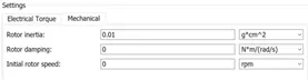
• Rotor Inertia: It’s a resistance of the rotor to change in motor motion.
• Rotor Damping: It should be zero because it is energy dissipated by the motor.
• Initial Rotor Speed: This is a starting speed of the motor that at what speed the motor will start.

Temperature Dependency

• Resistance temperature coefficient:93e-3 1/K
• Measurement temperature: 25 deg C

Thermal Port

• Thermal mass: 20000 J/K
• Initial temperature: 25 deg C

Thermal Port is connected with Temperature sensor Block to measure the motor temperature. Also, Ideal Rotational Motion Sensor is used to measure the motor speed.

H-BRIDGE & MOTOR CONTROLLER

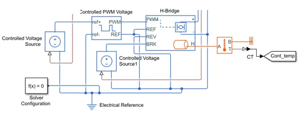
The H-Bridge block represents an H-bridge motor driver.

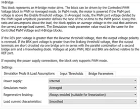
Simulation mode and Load Assumption Settings

• Power Supply: The power supply is default mode i.e. Internal.
• Simulation Mode: Here I selected Averaged mode and this mode has two Load current characteristics options:

 Smoothed

Unsmoothed or discontinuous

• Regenerative Braking: Always enabled (suitable for linearization), this option can be used when the controller always sets the REV flag to ensure regenerative braking.
• Load Current Characteristics: Smoothed, it’s a default option and it assumes that the current is practically continuous due to load inductance.

Input Thresholds

• Enable threshold voltage: 1.5 V, this is the above value of PWM at which H-Bridge start.
• PWM signal amplitude: 5.0 V, this is the amplitude of the signal at the PWM input. Here I used it as the default mode.
• Reverse threshold voltage: 1.5 V, here I changed this value.
• Braking threshold voltage: 2.5 V

Bridge Parameters

• Output voltage amplitude: 60.8 V, this parameter will be active only when we select Internal for Power Supply mode and it’s an amplitude of the voltage across the H-Bridge.
• Total bridge on resistance: 0.1 ohms,
• The freewheeling diode on resistance: 0.05 ohm
• Measurement Temperature: 25 degC

Temperature Dependency

• Total bridge on resistance at second measurement temperature:00001 ohm
• Freewheeling diode on resistance at second measurement temperature: 001 ohm
• Second measurement temperature:15 degC

Thermal Port

• Thermal mass: 20000 J/k
• Initial temperature: 25 degC

Detail about connection

• PWM: Pulse-width modulated signal.
• REF: Reference, it is an electrical conversing port associated with the floating zero volts.
• REV: Reverse, it is an electrical conserving port associated with the voltage that controls when to reverse the polarity of the H-Bridge block output.
• BRK: BRK, it is an electrical conserving port associated with the voltage that controls when to short circuit the H-Bridge block output.

Here PWM output port is connected with PWM input port of controlled PWM voltage. The REF and REV port are connected with REF port of controlled PWM voltage port. The BRK port is connected with a controlled voltage source.

The positive (+) terminal is connected with the positive (+) port of current sensor and negative (-) port is connected with the negative (-) port of DC motor.

Thermal port (H) is connected with temperature sensor to measure the temperature of controller.

CONTROLLED PWM VOLTAGE

The Controlled PWM Voltage block represents a pulse-width modulated (PWM) voltage source. The input detail is as given below.

Detail about the connection

• ref+ — Positive terminal, this port is a positive electrical reference and connected with controlled voltage source positive terminal.
• ref- — Negative terminal, this port is a negative electrical reference and connected with the negative terminal of the controlled voltage source.
• PWM — Pulse-width modulated signal, this port is electrical reference port and connected with PWM port of H-Bridge.
• REF — Floating zero-volt reference, this port is connected with REF and REV of H-Bridge port.

PWM Setting

• PWM frequency: 1000 Hz
• Sample time: 1e-6 s
• Input voltage for 100% duty cycle: 2 V
• Output voltage amplitude: 60.8 V

CONTROLLED VOLTAGE SOURCE

The Controlled Voltage Source block represents an ideal voltage source that is powerful enough to maintain the specified voltage at its output regardless of the current flowing through the source.

The block has one physical signal input port and two electrical conserving ports associated with its electrical terminals.

SOLVER CONFIGURATION

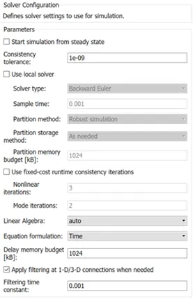
Solver configuration is used to begin the simulation and it is needed to solve the Simulink model. Here it is connected with controlled PWM voltage and H-Bridge negative connection by combination with electrical reference i.e ground signal.

Simulink Model of Electric Rickshaw :

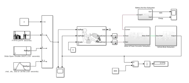
Simulink Explanation :

• Initially the current flows to DC Motor from the battery through the DC-DC power converter to drive the motor. The required voltage will be controlled in the controller. The Controller will follow the given drive cycle reference and run the motor in the required rpm.
• Then the motor power is transmitted to the wheels of a vehicle through the gear box. and the controller will take the vehicle speed and compare and controlled.

DISTANCE CALCULATION

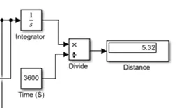
• Here the main block is an integrator, Divide, time block and for the result we have to use display block that will display the distance.
• Detail about connection:
• Integrator
• The output port of the vehicle body is connected with the integrator block.
• Divide
• The output of the integrator block is connected with divide where it will be divided by time to get the final output.
• Time
• The output of time block is connected with the divide block. Here time is taken as 3600 s.

RESULTS

Depending upon three drive cycle we will get following results.

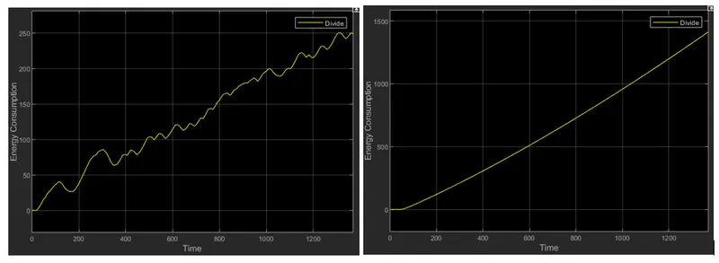
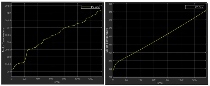
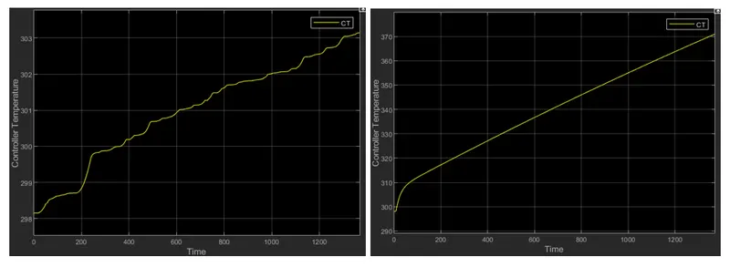
For UDDS drive cycle (Urban Dynamometer Driving Schedule) a vehicle run for 1369 sec and the total distance covered during this is 12.7404 km and at that time the energy consumption was 248.6 kW, Temperature rises in motor 302.2 degC and temperature rise in controller 303.1 degC.

Output Results based on ideal condition and PID Tunned. If we tunned the model then we will get following result as I have compared in table.

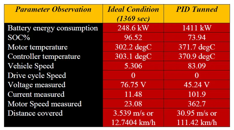
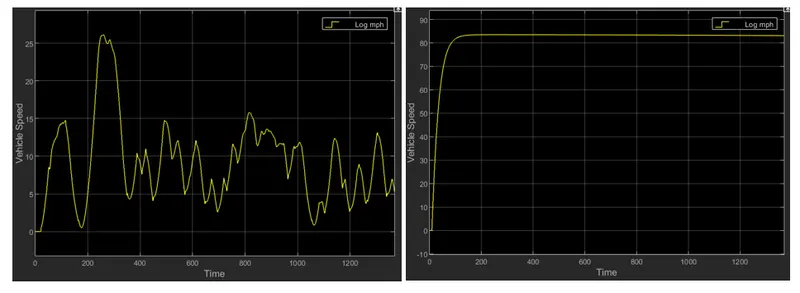
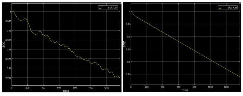
Plotted results: Ideal Condition Vs PID Tunned

Energy Consumption

Motor Temperature

Controller Temperature

Vehicle Speed

SOC

Distance

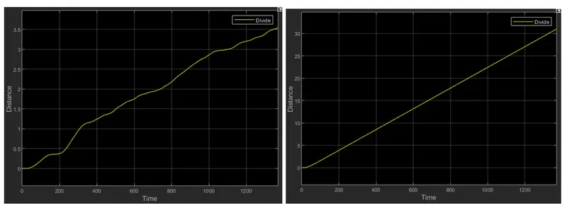
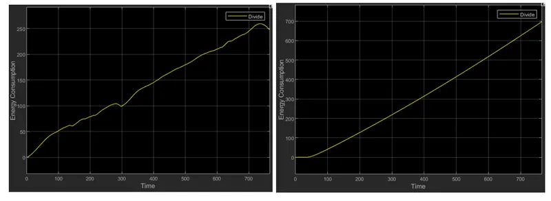
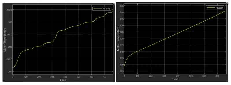
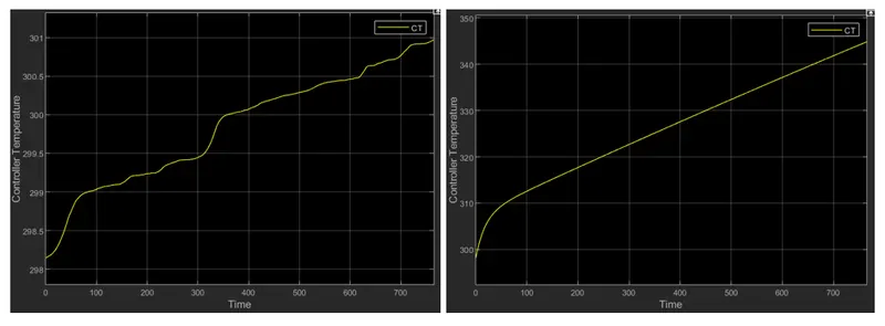
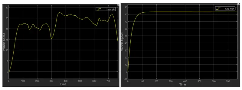
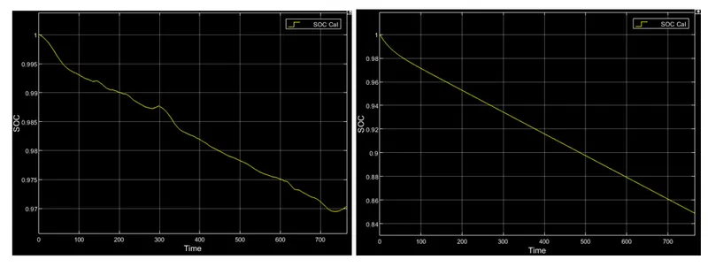
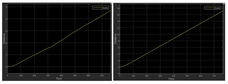
For HWFET drive cycle (Highway Fuel Economy Driving Schedule) a vehicle run for 765 sec and the total distance covered during this is 16.8552 km and at that time the energy consumption was 248 kW, Temperature rises in motor 300.4 degC and temperature rise in controller 301 degC.

Output Results based on ideal condition and PID Tunned. If we Tunned the model then we will get following result as I have compared in table.

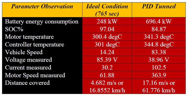
Plotted results: Ideal Condition Vs PID Tunned

Energy Consumption

 

Motor Temperature

 

Controller Temperature

 

Vehicle Speed

 

SOC

 

Distance

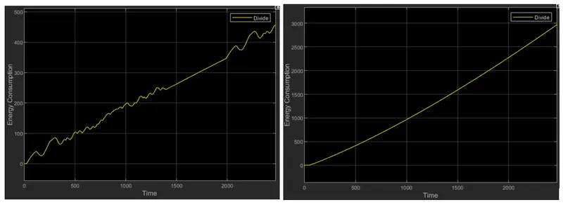
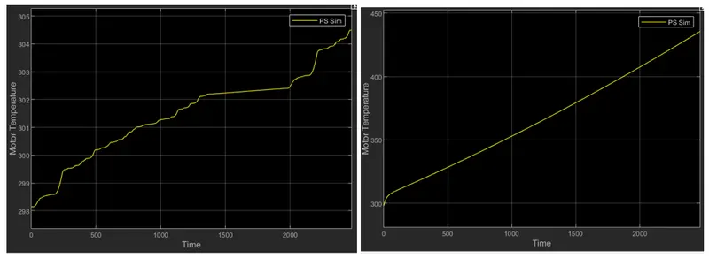
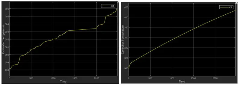
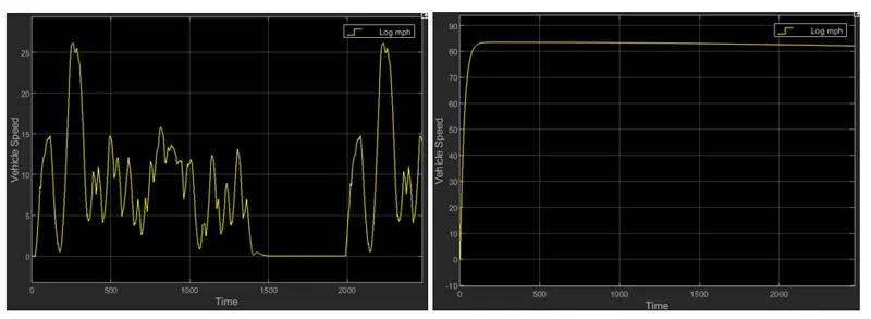
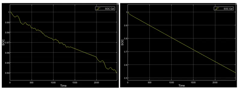
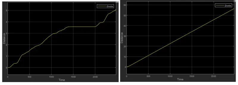
For FTP75 drive cycle a vehicle run for 2474 sec and the total distance covered during this is 18.2808 km and at that time the energy consumption was 455 kW, Temperature rises in motor 304.5 degC and temperature rise in controller 305.9 degC.

Output Results based on ideal condition and PID Tunned. If we Tunned the model then we will get following result as I have compared in table.

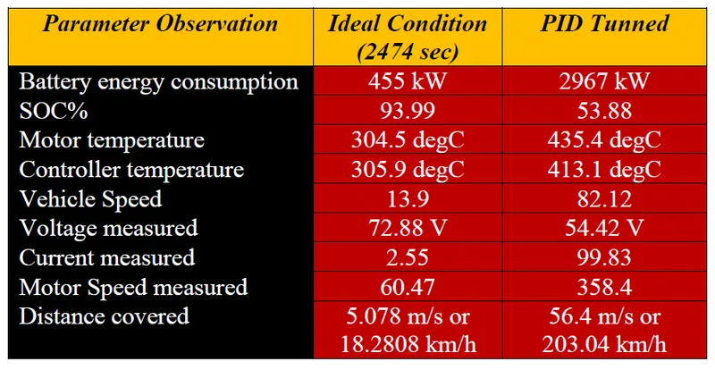
Plotted results: Ideal Condition Vs PID Tunned

Energy Consumption

 

Motor Temperature

 

Controller Temperature

 

Vehicle Speed

 

SOC

 

Distance

 

Conclusion:

• If we compare with real model then the motor, battery and controller temperature is controlled by using air cooling system because it is not high.
• The MATLAB model of e-rickshaw is created by using Li-ion Battery 60.8 V 160Ah and PM Brushed DC Motor.
• Also, after PID tunning the temperature is rises and we get better distance as compared with non-tunned electric rickshaw.