Final Project: Electric Rickshaw modelling

Question-

Create a detailed MATLAB model of an electric rickshaw (three wheel passenger vehicle) as per details below: 

Rear wheels driven by PM brushed type motor

Assume efficiency points of motor controller and motor

Make an excel sheet of all input and assumed data 

Results: For any three standard driving cycles show energy consumption, temperature rise of motor and controller for 100 km constant speed driving at 45 kmph.

(Note- The simulink model file should be compulsorily attached)

ANS:

AIM: Create a detailed MATLAB model of an electric rickshaw (three-wheel passenger vehicle) as per details below: 

• Rear wheels driven by PM brushed type motor
• Assume efficiency points of motor controller and motor
• Make an excel sheet of all input and assumed data.

ABSTRACT:

In this project, we going to build the MATLAB model of the electric rickshaw by using a PM brushed type DC motor and a suitable Lithium-Ion battery for the motor. Before that, we will know about what is electric rickshaw, how it's works and the benefits of EV Rickshaw. Then we make an actual EV Rickshaw model in SIMULINK with suitable blocks from the powertrain block set. My main motto is to check "how my Rickshaw performs for any three standard driving cycles showing energy consumption, the temperature rise of motor and controller for vehicle cover around 100 km at constant speed driving 45 kmph. Made a comparison with Mahindra e-Rickhaew and my Simulink model. 

OBJECTIVE:

•  To make the simple and low run-time vehicle model using the individual component model.
•  To check out performance parameters: Speed, SOC, current, the temperature of motor and H-bridge, etc. with various drive cycles.
•  To play with Motor power, vehicle body (Rolling resistance, Air drag, weight) inputs.
•  To know the MATLAB model and their configuration to match with the actual vehicle.

METHODOLOGY:

• The electric vehicle consists of a battery, motors, and controller then it generates propulsion power.
• To design any vehicle 1st we have to calculate propulsion power, then the motor is selected.
• Lastly based on the motor rating or operating range and no km/charge we want to depend on everything battery capacity and then battery capacity is selected.
• So the Design flow of vehicle engineer has to be like the following:

               1) Identify what amount of propulsion power required.

               2) What is the best suitable motor for that propulsion power.

               3) Then type of battery and range of battery according to the range.

THEORY: 

Electric rickshaws (also known as electric tuk-tuks or e-rickshaws or toto or e-tricycles) have been becoming more popular in some cities since 2008 as an alternative to the auto-rickshaws and pulled rickshaws because of their low fuel cost, and less human effort compared to pulled rickshaws. They are being widely accepted as an alternative to petrol, diesel, CNG auto-rickshaws. They are three-wheelers powered by an Electric motor ranging from 650 to 1400  Watts. They are mostly manufactured in India and China, only a few other countries manufacture these vehicles. Battery-run rickshaws could be a low-emitter complimentary transport for the low-income people, who suffer most from a lack of transport facility if introduced in a systematic manner according to experts.

Development of the E-rickshaw market in India:

E-Rickshaw's have now transitioned from being a market entrant in the automobile segment of the country to evolve as a leading short-distance transport solution. This segment has gained a spurt in the last three years and the growth has been phenomenal. Although, this segment is dominated by a host of unorganized players the established names have also identified the growth beacon and are expected to foray into the segment. One of the first attempts to design electric rickshaws was done by Nimbkar Agricultural Research Institute in the late 1990s.In India, this so-called e-rickshaws are widely spread all over the country, starting to gain popularity around 2011. The design is now much different from cycle rickshaws. Today, e-rickshaws play a vital role in providing livelihood to people in India. Due to their low cost and high efficiency, they are accepted on the Indian streets, but government policies have been threatening the e-rickshaw and banned its use in the capital city Delhi but failed to put them off the streets. E-rickshaws are still rising in number and widely used in Delhi and other parts of India. In Delhi, as per government official's figures in April 2012, their number was over 100,000.

Design and Construction:

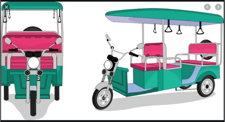
These rickshaws have an M.S(Mild Steel) tubular chassis, consisting of three wheels with a differential mechanism at the rear wheels. The motor is a brushless DC motor manufactured mostly in India and China. The electrical system used in the Indian version is 48V and in Bangladesh is 60V. The body design from the most popular Chinese version is of very thin iron or aluminum sheets. Vehicles made in fiber are also popular because of their strength and durability, resulting in low maintenance, especially in India. The body design is varied from load carriers, passenger vehicles with no roof, to full body with windshield for drivers comfort. It consists of a controller unit. They are sold on the basis of voltage supplied and current output, also the number of MOSFET (metal oxide field-effect transistors) used. The battery used is mostly a lead-acid battery with life of 6–12 months. Deep cycle batteries designed for electric vehicles are rarely used. The weight of the electric car has also been a recurring design difficulty in them.

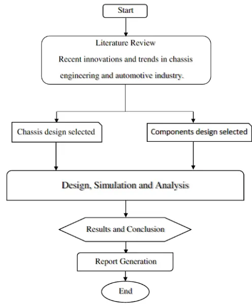
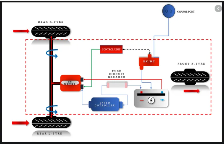
Below shows the methods followed throughout:

PROCEDURE: 

1) Identify what amount of propulsion power required 

2) What is the best suitable motor for that propulsion power.

3) Then type of battery and range of battery according to the range.

Why we should be required to calculate 1st propulsion power?

The final outcome of the vehicle is propulsion power and therefore the start point should be what is propulsion power on the calculation of proper power, therefore, the study must begin with an estimation of propulsion power.

Why we should Disgne 1st instead of directly build the model of EV?

This mathematical model must be build before making an actual hardware design so this model offers great flexibility in conceptual design modification. For example, If I changed the components, you can do it easily in a mathematical model rather than in actual mode and check its parameters.

This model gives the performance idea with reasonable accuracy and avoided repetitive road tests. Models are very helpful in many situations can be realized safely only in analysis and calculation i.e .. thermal.

Yes, there are limitations of mathematical models also it is really difficult to implement all the aspects involves so those models are with certain assumptions with certain inaccuracies. But more and more aspects you covered the more and more benefit and accuracy will get.

* Now we start to design the model from zero like from Wheel, vehicle body, then we get to the motor, battery and it will be full powertrain.

so we divided our model into some part as below:

                                               1) Wheel and vehicle body (mechanical part).

                                               2) Electric system.

                                               3) Battery System and SOC.

                                               4) Controller.

                                               5) Inputs.

Wheel and vehicle body:

For wheel and vehicle body we have to consider the following parameters 

Force acting on the vehicle- 1) To bring the vehicle to accelerate. 2) To maintain that speed.  

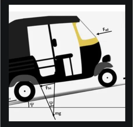
Where,

1)  ψ= Angle.

2)fte= tractive force.

3)frr= Rolling resistance force.

4)fad= Airo dynamic drag force.

5)fhc= Hill climbing force.

In the above fig.

fte=Frr+Fad+Fhc+acceleration force

Two type of acceleration force is their linear acceleration force and angular acceleration force.

Rolling resistance force:                 

The rolling resistance can be expressed by the generic equation

Fr = c W                               (1)

where

Fr = rolling resistance or rolling friction (N, lbf)

c = rolling resistance coefficient - dimensionless (coefficient of rolling friction - CRF)

W = m ag

= normal force - or Weight - of the body (N, lbf)

m = mass of body (kg, lb)

ag = acceleration of gravity  (9.81 m/s2, 32.174 ft/s2)

Note that the rolling resistance coefficient - c - is influenced by different variables like wheel design, rolling surface, wheel dimensions and more.

The rolling resistance can alternatively be expressed as

Fr = cl W / r                            (2)

where

cl = rolling resistance coefficient - dimension length (coefficient of rolling friction) (mm, in)

r = radius of wheel (mm, in)

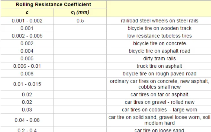
Some typical rolling coefficients:

http://ffden-2.phys.uaf.edu/webproj/212_spring_2017/Ethan_Trickey/Ethan_Trickey/1st%20page.html

Aerodynamic drag force:

This force considers the shape drag and skin friction basically for doby of vehicle.

This force function of the frontal area, shape, side mirror, ducts, air passage, etc.

                              Fad= 1/2⋅ρ⋅A⋅Cd⋅V^2 

Where,

ρ= Air density(kg/m^3)

A =Frontal area(m^2)

Cd= drag coefficient.

V= velocity(m/s)

Hill climbing force:

                               Fhc=m.g.sinψ

Where,

m = mass of body (kg, lb)

g=gravity  (9.81 m/s2)

sinψ=Slop angle.

This force Is also represented by using gradeability. Gradeability can overcome by vehicle constant speed. There are two ways 1) degree            2) percentage

The power output by the car's engine goes into the force-directed up the slope. This force is actually static friction exerted on the drive wheels by the road - the road exerts this force F because the engine causes the drive wheels to rotate. 

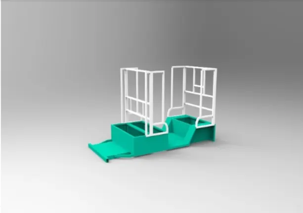
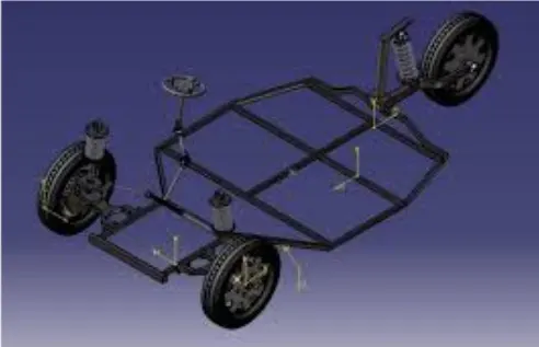
By considering all parameters we can know the design of the vehicle body and Wheel of the rickshaw.

Body:

Wheel:

So we selected the following block for tire and vehicle body:

 

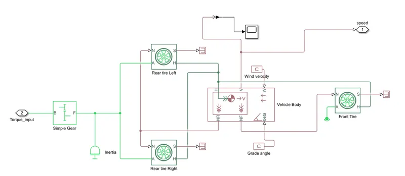
In the above body and tire model following blocks are used:

1) Tire (Magic Formula): 

Represents the longitudinal behavior of a highway tire characterized by the tire Magic Formula. The block is built from Tire-Road Interaction (Magic Formula) and Simscape Foundation Library Wheel and Axle blocks. Optionally, the effects of tire inertia, stiffness, and damping can be included.

A is the mechanical rotational conserving port for the wheel axle

H is the mechanical translational conserving port for the wheel hub through which the thrust developed by the tire is applied to the vehicle.

N is a physical signal input port that applies the normal force acting on the tire.

S is a physical signal output port that reports the tire slip. 

So this is a car we need 4 wheel and this tire ports connected to the appropriate signal as mention above.

Following parameters considered for tire:

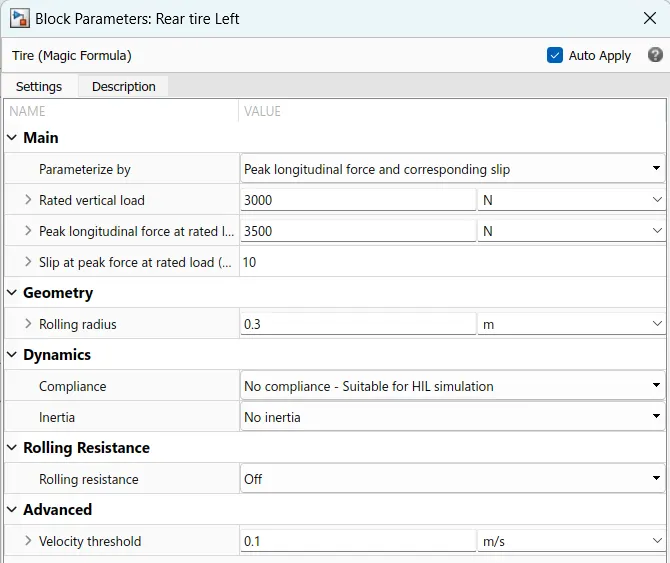
Now we just take the default values to check how they perform but we can take parameters of the currently existing rickshaws.   

2) Vehicle Body:

Represents a two-axle vehicle body in longitudinal motion. The block accounts for body mass, aerodynamic drag, road incline, and weight distribution between axles due to acceleration and road profile. The vehicle can have the same or a different number of wheels on each axle. Optionally include pitch and suspension dynamics or additional variable mass and inertia.

H is the mechanical translational conserving port associated with the horizontal motion of the vehicle body. The resulting traction motion developed by tires should be connected to this port.

V, NF, and NR are physical signal output ports for vehicle velocity and front and rear normal wheel forces, respectively.

W and beta are physical signal input ports corresponding to headwind speed and road inclination angle, respectively.

Following parameters considered for vehicle body:

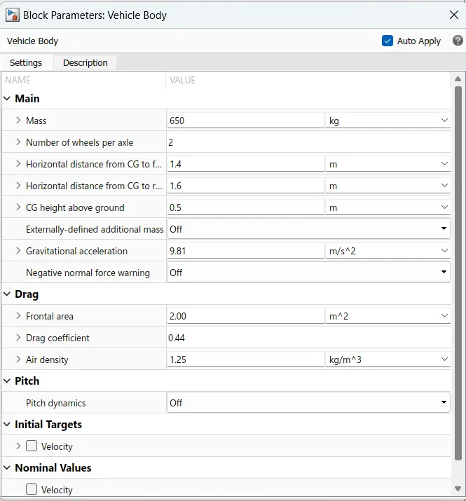
PS constant:

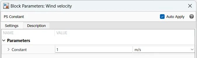
This block creates a physical signal constant:

y = constant

The Constant parameter accepts both positive and negative values. The block output is a physical signal port.

This PS constant is connected to the Vehicle body port W and delt for we can change the value of angel and wind velocity but we kept this value now zero.

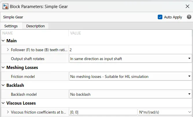
Simple Gear:

    

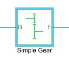
Represents a fixed-ratio gear or gear box. No inertia or compliance is modeled in this block. You can optionally include gear meshing, backlash, and viscous bearing losses.

Connections B (base) and F (follower) are mechanical rotational conserving ports. Specify the relation between base and follower rotation directions with the Output shaft rotates parameter. Optionally include thermal effects and expose thermal conserving port H by setting Friction model to a temperature-dependent setting.

Electric system:

Depending upon the tractive force, Environmental conditions, type of vehicle application we choose the motor for the vehicle. For that motor, we will decide the controller 

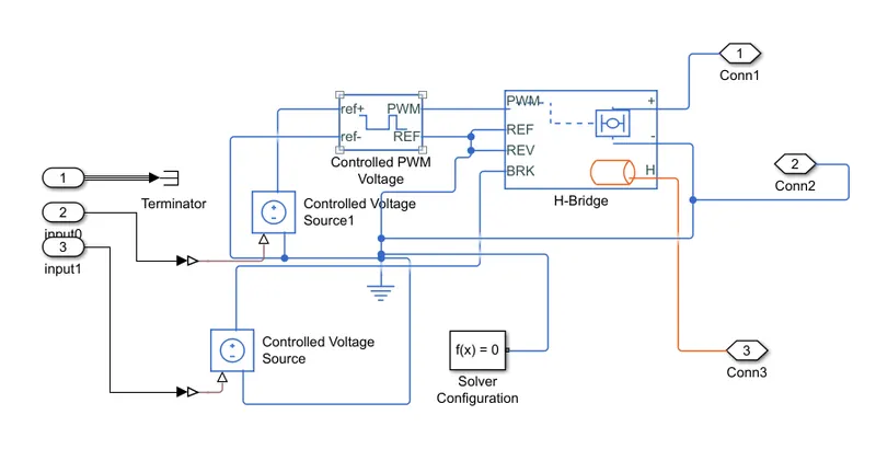
In Electric system Included the Motor, H-Bridge, controlled  PWM voltage.

As per our Aim, we using the PM brushed DC motor and for that motor, we used DC to Dc converter which is H-bridge.

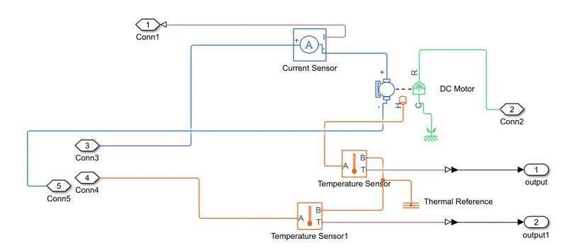
Following is my Electric model used in this EV model:

To build this model we used the following blocks and parameters changed in it:

1)DC motor:

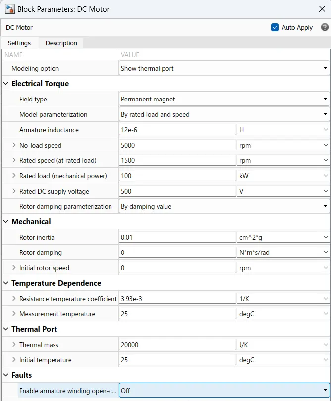
This block represents the electrical and torque characteristics of a DC motor. The block assumes that no electromagnetic energy is lost, and hence the back-emf and torque constants have the same numerical value when in SI units. Motor parameters can either be specified directly or derived from the no-load speed and stall torque. If no information is available on armature inductance, this parameter can be set to some small non-zero value. 

When a positive current flows from the electrical + to - ports, a positive torque acts from the mechanical C to R ports. Motor torque direction can be changed by altering the sign of the back-emf or torque constants.

Following parameters, we used for this Ev model:

Thermal Port:

The block has an optional thermal port, hidden by default. To expose the thermal port, right-click the block in your model, and then from the context menu select Simscape > Block choices > Show thermal port. This action displays the thermal port H on the block icon, and exposes the Temperature Dependence and Thermal Port parameters.

Use the thermal port to simulate the effects of copper resistance losses that convert electrical power to heat. For more information on using thermal ports and on the Temperature Dependence and Thermal Port parameter.

Thermal sensor:

         

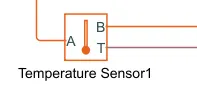
This block measures temperature in a thermal network. There is no heat flow through the sensor. The physical signal port T reports the temperature difference across the sensor. The measurement is positive when the temperature at port A is greater than the temperature at port B.

DC motor with controller:

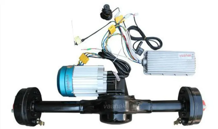
H-bridge:

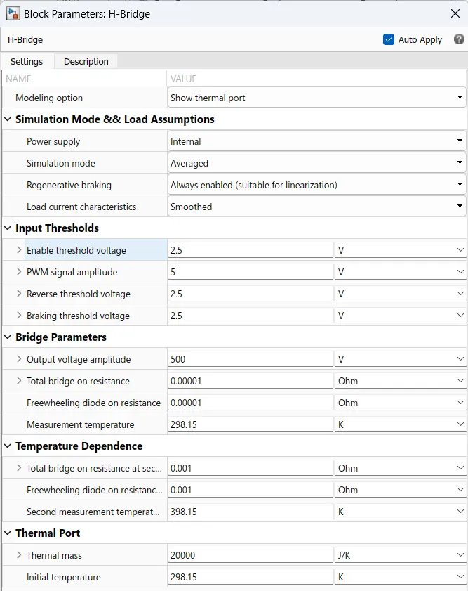
This block represents an H-bridge motor drive. The block can be driven by the Controlled PWM Voltage block in PWM or Averaged mode. In PWM mode, the motor is powered if the PWM port voltage is above the Enable threshold voltage. In Averaged mode, the PWM port voltage divided by the PWM signal amplitude parameter defines the ratio of the on-time to the PWM period. Using this ratio and assumptions about the load, the block applies an average voltage to the load that achieves the correct average load current. The Simulation mode parameter value must be the same for the Controlled PWM Voltage and H-Bridge blocks.

If the REV port voltage is greater than the Reverse threshold voltage, then the output voltage polarity is reversed. If the BRK port voltage is greater than the Braking threshold voltage, then the output terminals are short-circuited via one bridge arm in series with the parallel combination of a second bridge arm and a freewheeling diode. Voltages at ports PWM, REV, and BRK are defined relative to the REF port.

The following parameters are selected for H-bridge:

Thermal Port:

The block has an optional thermal port, hidden by default. To expose the thermal port, right-click the block in your model, and then from the context menu select Simscape > Block choices > Show thermal port. This action displays the thermal port H on the block icon, and adds the Temperature Dependence and Thermal Port parameters. These parameters are described further on this reference page.

When the thermal port is visible:

• The heat generated by the bridge on-resistance and freewheeling diodes is added to the thermal port. The thermal port has an associated thermal mass and initial temperature that you can set from the Thermal Port parameters.
• The bridge on-resistance and freewheeling diode resistance become functions of temperature. You can define the values for these resistances and the second measurement temperature from the Temperature Dependence parameters. Resistance is assumed to vary linearly between the two measurement temperatures. Extrapolation is used for temperatures outside of this range, except for when simulating in averaged mode with discontinuous load current characteristics.

Controlled PWM voltage:

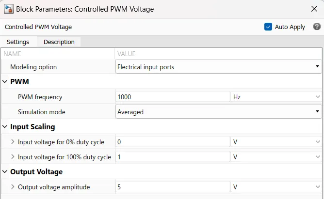
This block creates a Pulse-Width Modulated (PWM) voltage across the PWM and REF ports. The output voltage is zero when the pulse is low and is equal to the Output voltage amplitude parameter when high. The duty cycle is set by the input value. Right-click the block and select Simscape-Block choices to switch between electrical +ref/-ref ports and PS input u to specify the input value. At time zero, the pulse is initialized as high unless the duty cycle is set to zero or the Pulse delay time is greater than zero. 

The Simulation mode can be set to PWM or Averaged. In PWM mode, the output is a PWM signal. In Averaged mode, the output is constant with a value equal to the averaged PWM signal. 

Electrical input ports — The block calculates the duty cycle based on the reference voltage across its ref+ and ref- ports. This modeling variant is the default. 

PS input — Specify the duty cycle value directly by using an input physical signal port.

Following parameters used in Controlled PWM voltage:

Controlled voltage source:

The block represents an ideal voltage source that is powerful enough to maintain the specified voltage at its output regardless of the current passing through it. The output voltage is V = Vs, where Vs is the numerical value presented at the physical signal port.

Electrical Reference: 

Electrical reference port. A model must contain at least one electrical reference port (electrical ground).

Current sensor:

The block represents an ideal current sensor, that is, a device that converts current measured in any electrical branch into a physical signal proportional to the current.

Connections + and - are conserving electrical ports through which the sensor is inserted into the circuit. Connection I is a physical signal port that outputs the current value.

Battery System and SOC:

To need power for motor and other equipment we give battery pack. This battery pack is decided from a rating of the motor and considering another electric load. So we used a Lithium battery :

              

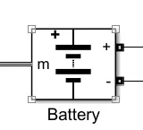
Implements a generic battery model for the most popular battery types. Temperature and aging (due to cycling) effects can be specified for Lithium-Ion battery type.

The Battery block implements a generic dynamic model that represents the most popular types of rechargeable batteries.

This figure shows the equivalent circuit that the block models.

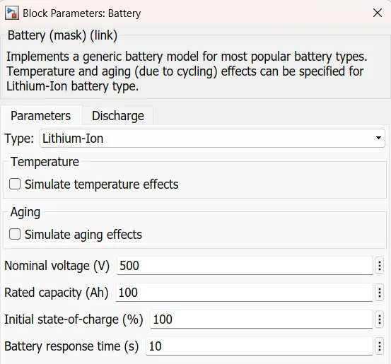
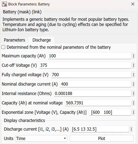
Battery Parameters:

Powergui:

The powergui block allows you to choose one of these methods to solve your circuit:

• Continuous, which uses a variable-step solver from Simulink®
• Discretization of the electrical system for a solution at fixed time steps
• Continuous or discrete phasor solution

The powergui block also opens tools for steady-state and simulation results analysis and for advanced parameter design.

You need the powergui block to simulate any Simulink model containing Simscape™ Electrical™ Specialized Power Systems blocks. It stores the equivalent Simulink circuit that represents the state-space equations of the model.

When using one powergui block in a model:

• Place the powergui block in the top-level diagram for optimal performance.

Make sure that the block is named powergui.

(SOC)  the state of charge estimator:

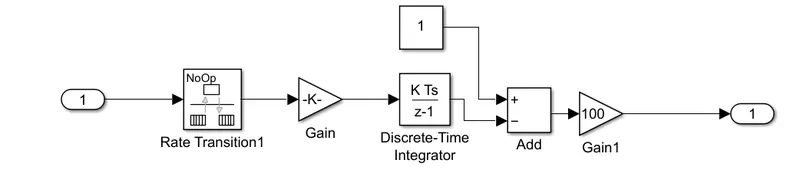
This estimator includes the above block which explained below:

Rate Transition: Handle data transfer between different rates and tasks.

Gain: Element-wise gain (y = K.*u) or matrix gain (y = K*u or y = u*K). Where we used an 60v battery so our formula is like 1/60*3600)

Discrete-time Integrator: Discrete-time integration or accumulation of the input signal.

Scope: to get the result of SOC, Current.

PS Simulink converter: Converts the input Physical Signal to a Simulink output signal.

Longitudinal Driver :

• Longitudinal Driver is an inbuilt block provided by the powertrain blockset.

                  

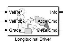
• It is a parametric longitudinal speed tracking controller for generating normalized Acceleration and Braking commands based on reference and feedback velocities.
• The VelFdbk port corresponds to the feedback velocity. The actual velocity output given by the vehicle body is connected here. By comparing the actual (feedback) velocity with the reference velocity, the driver block generates acceleration and braking signals in order to minimise the error between the two concerned velocities.
• Grade corresponds to the grade angle. For this simulation, no inclination is considered and hence, a constant block with value 1 is connected.
• Info gives the output for the bus signal for different block calculations like difference in reference vehicle speed and vehicle speed, etc.
• AccelCmd & DecelCmd correspond to the acceleration and deceleration commands generated respectively and are connected to the corresponding ports of the Controlled PWM Voltage block.
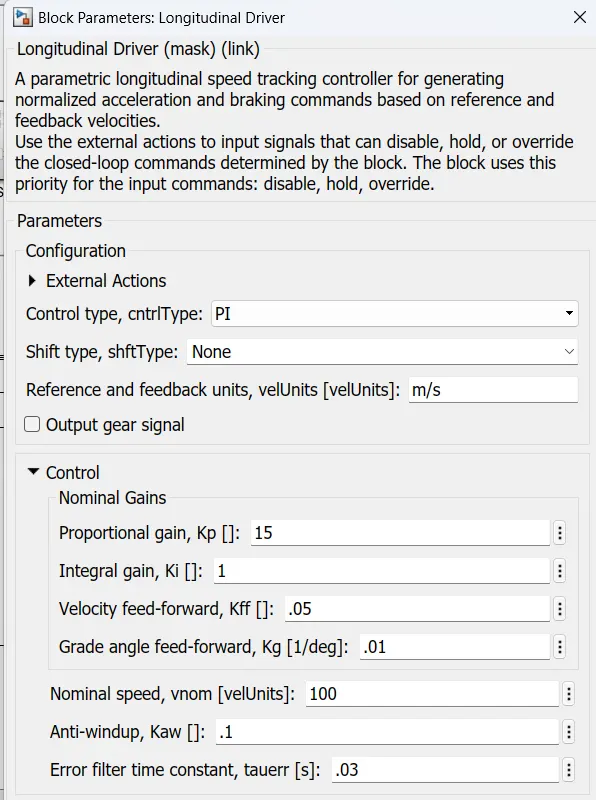
• Here, the selected control type is PI. Acordingly, the block implements proportional-integral (PI) control with tracking windup and feed-forward gains.

Reference Velocity (Drive Cycle) :

For the Control and input of hole EV model, we give input which is Drive cycle, Signal Bilder, WOT, etc.

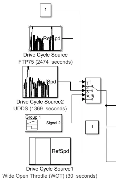
For the selection of these Inputs, we used multiple switches:

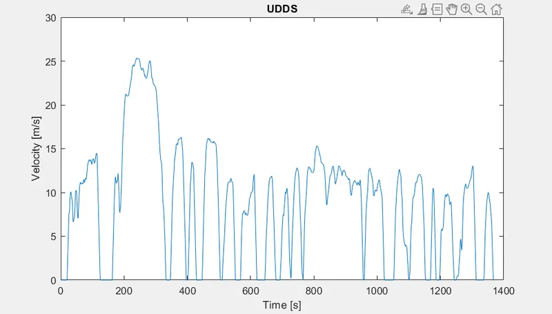
• Drive cycle is assumed as the driver's input of a vehicle, it replaced how a driver will drive a vehicle. Here I have used three drive cycles which is used to test the vehicle performances. These drive cycle will have high speed, low speed, braking conditions in it.
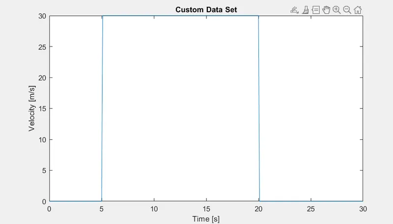
• There are different drive cycles like WOT, FTP75 etc., Here in this model I have used FTP 75, WOT & Manually prepared in excel Drive Cycle source. 

 FTP 75 :

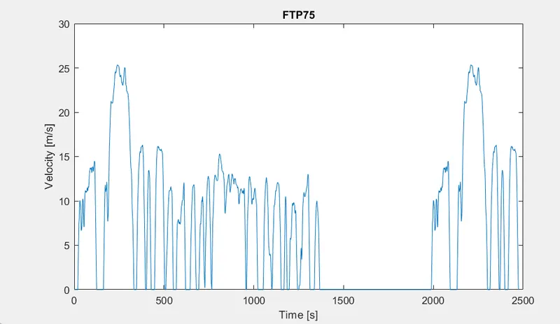
Generates a standard or user-specified longitudinal drive cycle. The block output is the vehicle longitudinal speed. You can import drive cycles from :

• Predefined sources
• Workspace variables, including arrays and time series objects
• mat, xls, xlsx, or txt files

Use the fault tracking parameters to identify drive cycle faults within specified speed and time tolerances.

Wide Open Throttle (WOT) :

UDDS:

 

• All 3 Drive cycles are controlled by the controller provided above by constant through Multi-port switch.

Simulink Model of Electric Rickshaw :

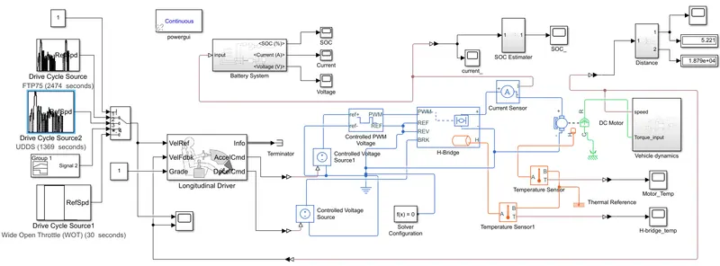
Simulink Explanation :

• Initially the current flows to DC Motor from the battery through the DC-DC power converter to drive the motor. The required voltage will be controlled in the controller. The Controller will follow the given drive cycle reference and run the motor in the required rpm.
• Then the motor power is transmitted to the wheels of a vehicle through the gear box. and the controller will take the vehicle speed and compare and controlled.

Output Plots :

 1. For FTP75 Drive Cycle :

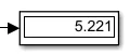
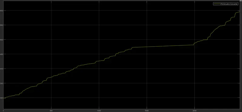
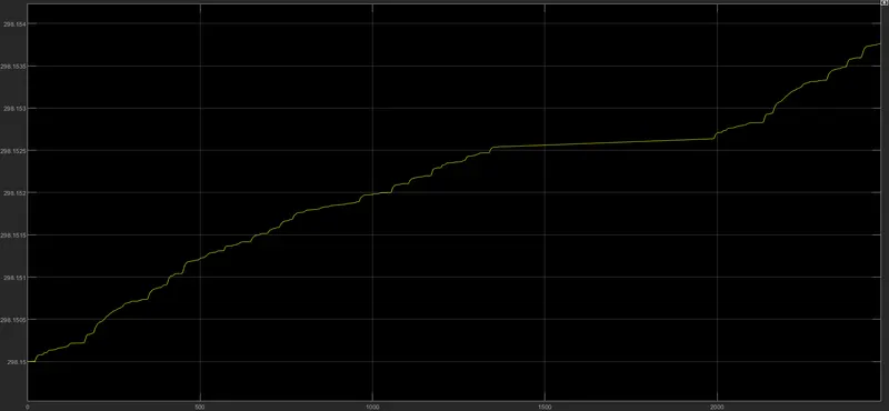
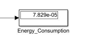
• By running the Vehicle with FTP75 Drive cycle for 2474 sec. the distance travelled is 5.221 km.

                  

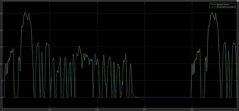
In this graph, we get the reference speed(yellow), the Output speed (blue)of the rickshaw. 

As we saw in the result we can check the my all graph is following the reference path as we required.

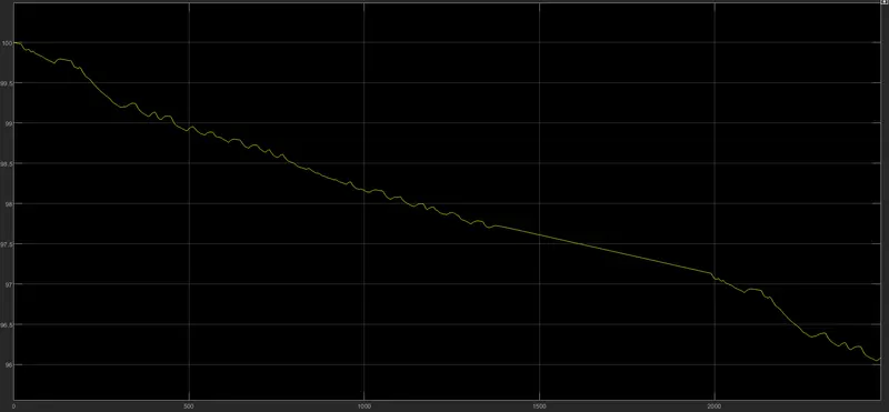
state of charge result:

The temperature of motor:

The temperature of Controller:

Energy Consumed:

                  

2. For UDDS Drive Cycle :

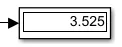
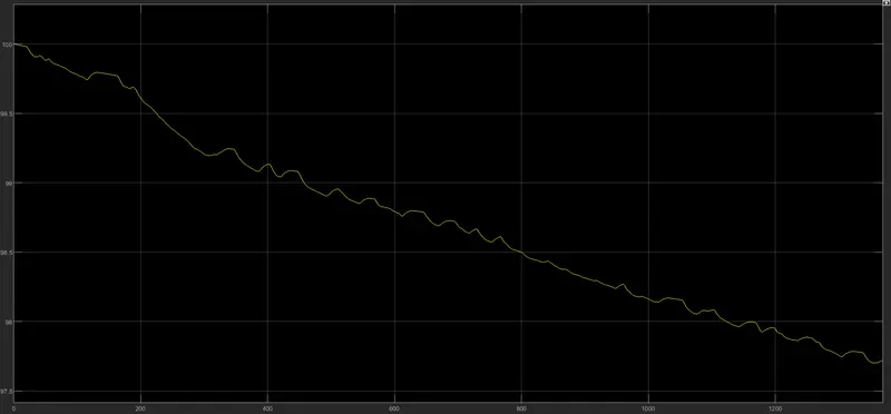
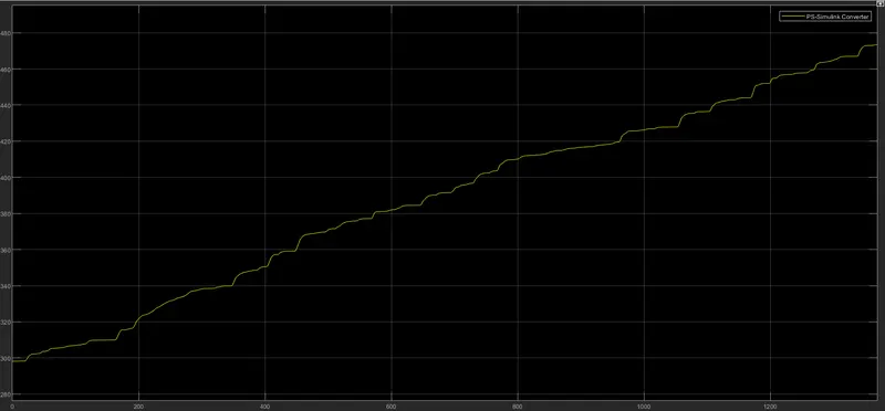
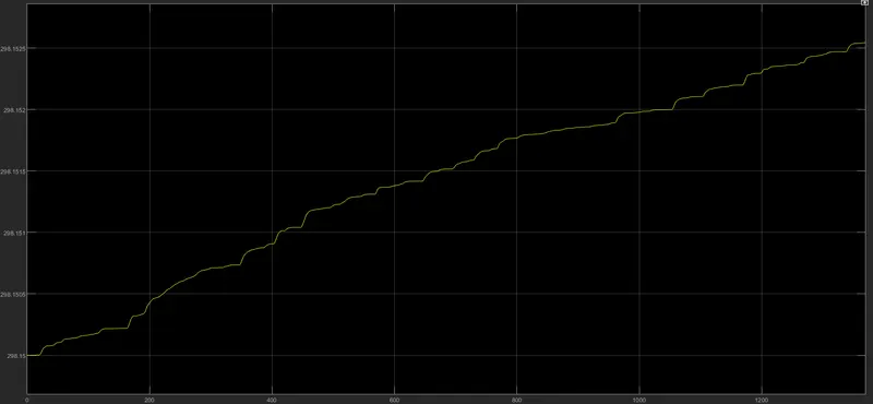
• By running the Vehicle with UDDS Drive cycle for 1369 sec. the distance travelled is 3.525 km.

                  

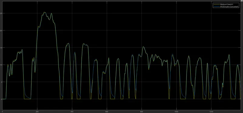
As we saw in the result we can check the my all graph is following the reference path as we required.

state of charge result:

The temperature of motor:

The temperature of Controller:

Energy Consumed:

3. For WOT Drive Cycle :

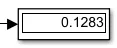
• By running the Vehicle with WOT Drive cycle for 30 sec. the distance travelled is 0.1283 km.

   

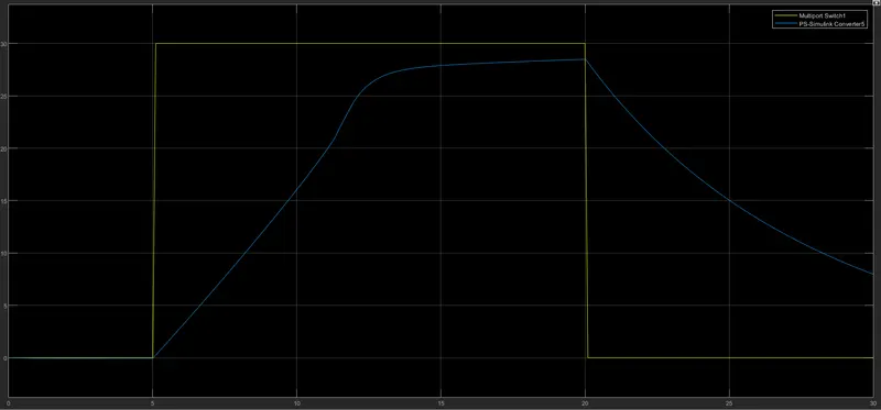
As we saw in the result we can check the my all graph is following the reference path as we required.

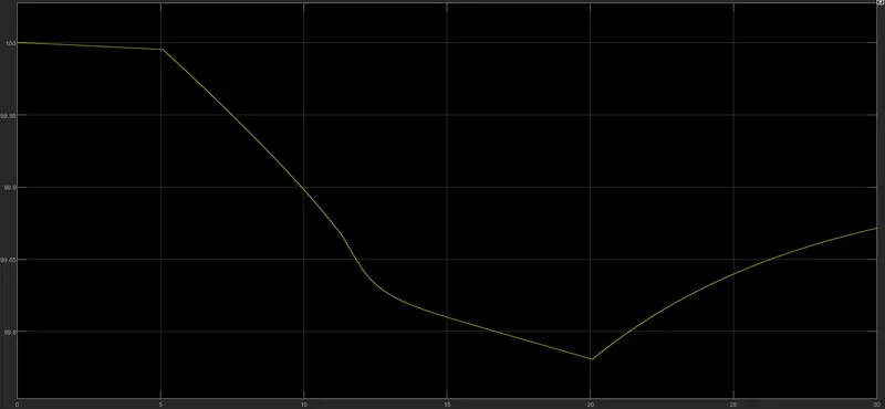
state of charge result:

The temperature of motor:

 

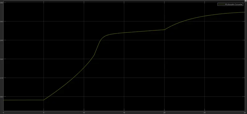
The temperature of Controller:

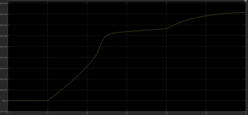
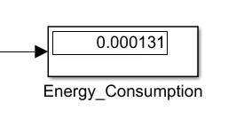
Energy Consumed:

              

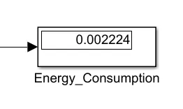
4) 100 km constant speed driving at 45 kmph:

For requirement meet, we are going to run the model for WOT but this time we give the top speed and second by calculation. By calculation, we get that the top speed is 12.5 mps and the second required is 28600 from this value we will get our requirement 100km distance with Constance speed of 45kmph(12.5 m/sec)

Signal Builder Input:

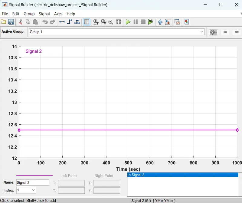
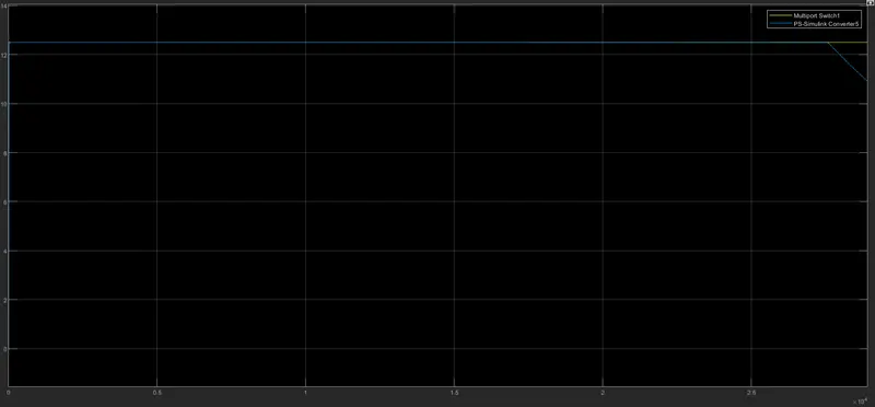
we can check the my all graph is following the reference path as we required.

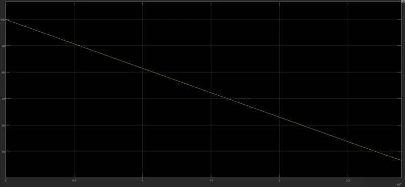
state of charge result:

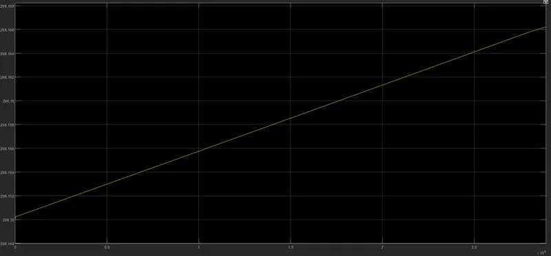
The temperature of Controller:

The temperature of motor:

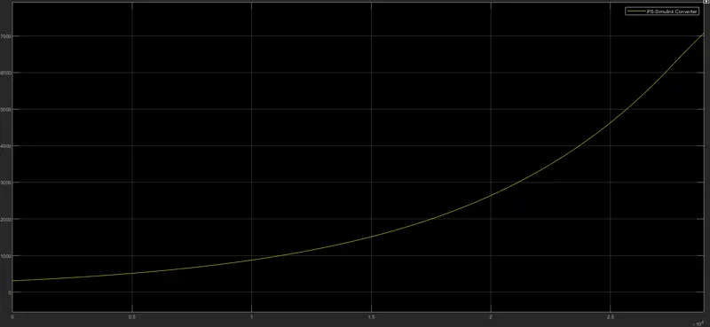
Energy Consumed:

                   

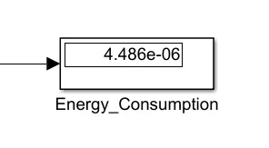
After the simulation run for time 28900 model cover a distance of around 100 km.

as we can see in SOC, the battery charge only in a reduced manner and it is in negative also that show that battery capacity has to increase. In practical battery may be burned for this condition.

Input Assumed Data:

CONCLUSION :

• Here I have compromised with the temperature of Motor and controller to achieve vehicle speed is near to reference speeds. Since I haven’t used any cooling system in the model. In the real time application, the motor temperature is less than 100 C.
• In the real time application, the motor, battery & controller temperature is controlled by air cooling. Hence, the temperature of this components is not increased to this extent.
• Hence, Created a MATLAB model of an Electric Rickshaw (three wheel passenger vehicle) by using Li-ion battery, PM Brushed DC Motor.
• Determined the variations of Temperature of Motor and controller, SoC% and Energy consumed by the by vehicle for all four Reference Drive cycles (i.e.; FTP75,UDDS, WOT, Manually prepared).
• This Battery powered Rickshaw will be the most popular mode of transport in the future.