Final Project: Electric Rickshaw modelling
Objectives:- Create a detailed MATLAB model of an electric rickshaw (three wheel passenger vehicle) as per details below:
Rear wheels driven by PM brushed type motor
Assume efficiency points of motor controller and motor
Make an excel sheet of all input and assumed data
Results: For any three standard driving cycles show energy consumption, temperature rise of motor and controller for 100 km constant speed driving at 45 kmph.
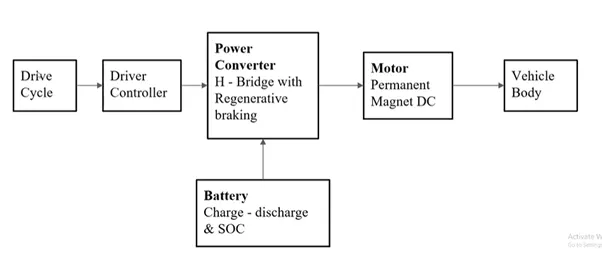
Block Diagram:-
Simulink Model Of an Electric Rickshaw:-
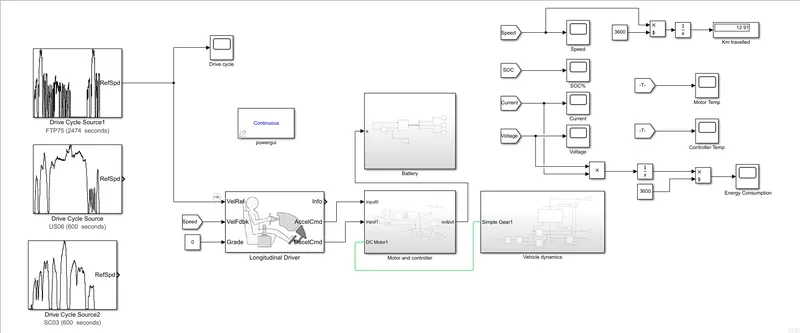
The Model Consists of a Drive Cycle, a Driver, Controller, Battery Pack, Motor and The Vehicle body. All the things such as SOC%, current, voltage, speed, Distance Travelled and Temperature of the Motor and Controller will be observed.
Block Parameters:-
Drive Cycle:-
FTP-75
The "city" driving program of the EPA Federal Test Procedure is identical to the UDDS plus the first 505 seconds of an additional UDDS cycle.
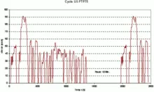
EPA FTP-75 driving cycle
Then the characteristics of the cycle are:
- Distance travelled: 17.77 km (11.04 miles)
- Duration: 1874 seconds
- Average speed: 34.1 km/h (21.2 mph)
The procedure is updated by adding the "hot start" cycle that repeats the "cold start" cycle of the beginning of the UDDS cycle. The average speed is thus different but the maximum speed remains the same as in the UDDS. The weighting factors are 0.43 for the cold start and transient phases together and 0.57 for the hot start phase.
Though it was originally created as a reference point for fossil fuelled vehicles, the UDDS and thus the FTP-75, are also used to estimate the range in distance travelled by an electric vehicle in a single charge
US06
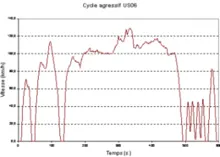
EPA US06 supplemental driving cycle
The US06 Supplemental Federal Test Procedure (SFTP) was developed to address the shortcomings with the FTP-75 test cycle in the representation of aggressive, high speed and/or high acceleration driving behaviour, rapid speed fluctuations, and driving behaviour following start up.
SFTP US06 is a high speed/quick acceleration loop that lasts 10 minutes, covers 8 miles (13 km), averages 48 mph (77 km/h) and reaches a top speed of 80 mph (130 km/h). Four stops are included, and brisk acceleration maximizes at a rate of 8.46 mph (13.62 km/h) per second. The engine begins warm and air conditioning is not used. Ambient temperature varies between 68 °F (20 °C) to 86 °F (30 °C).
The cycle represents an 8.01 mile (12.8 km) route with an average speed of 48.4 miles/h (77.9 km/h), maximum speed 80.3 miles/h (129.2 km/h), and a duration of 596 seconds.
SC03
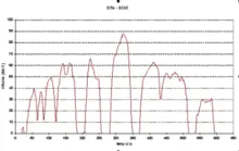
EPA SC03 supplemental driving cycle
The SC03 Supplemental Federal Test Procedure (SFTP) has been introduced to represent the engine load and emissions associated with the use of air conditioning units in vehicles certified over the FTP-75 test cycle.
SFTO SC03 is the air conditioning test, which raises ambient temperatures to 95 °F (35 °C), and puts the vehicle's climate control system to use. Lasting 9.9 minutes, the 3.6-mile (5.8 km) loop averages 22 mph (35 km/h) and maximizes at a rate of 54.8 mph (88.2 km/h). Five stops are included, idling occurs 19 percent of the time and acceleration of 5.1 mph/sec is achieved. Engine temperatures begin warm.
The cycle represents a 3.6 mile (5.8 km) route with an average speed of 21.6 miles/h (34.8 km/h), maximum speed 54.8 miles/h (88.2 km/h), and a duration of 596 seconds.
Longitudinal Driver:-
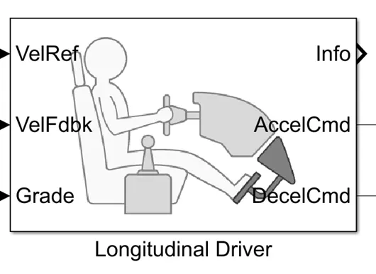
The Longitudinal Driver block implements a longitudinal speed-tracking controller. Based on reference and feedback velocities, the block generates normalized acceleration and braking commands that can vary from 0 through 1. You can use the block to model the dynamic response of a driver or to generate the commands necessary to track a longitudinal drive cycle.
Motor & Controller Block:-
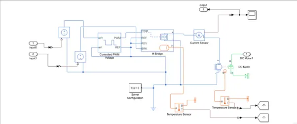
The Input from the Driver block is fed into this block. The Acceleration input from the driver is given to the ‘ref+’ of the Controlled PWM voltage which in turn gives the PWM signal to the controller and the Braking input is directly given to the ‘BRK’ terminal of the H-Bridge.
Controlled PWM Voltage:-
The Controlled PWM Voltage block represents a pulse-width modulated (PWM) voltage source. The block has two modeling variants, accessible by right-clicking the block in your block diagram and then selecting the appropriate option from the context menu, under Simscape > Block choices:
- Electrical input ports— The block calculates the duty cycle based on the reference voltage across its ref+ and ref- This modeling variant is the default.
- PS input— Specify the duty cycle value directly by using an input physical signal port.
For the Electrical input ports variant of the block, the demanded duty cycle is
`100* (V_(ref) – V_min)/(V_max – V_min)`
where:
- Vrefis the reference voltage across the ref+ and ref-
- Vminis the minimum reference voltage.
- Vmaxis the maximum reference voltage.
The value of the Output voltage amplitude parameter determines amplitude of the output voltage.
At time zero, the pulse is initialized as high, unless the Pulse delay time parameter is greater than zero, or the demanded duty cycle is zero.
You can use parameters Pulse delay time and Pulse width offset to add a small turn-on delay and a small turn-off advance. This can be useful when fine-tuning switching times so as to minimize switching losses.
In PWM mode, the block has two options for the type of switching event when moving between output high and output low states:
- Asynchronous – Best for variable-step solvers— Asynchronous events are better suited to variable step solvers, because they require fewer simulation steps for the same level of accuracy. In asynchronous mode the PWM switching events generate zero crossings, and therefore switching times are always determined accurately, regardless of the simulation maximum step size.
- Discrete—time – Best for fixed-step solvers— Discrete-time events are better suited to fixed-step operation, because then the switching events are always synchronized with the simulation step. Using an asynchronous implementation with fixed-step solvers may sometimes result in events being up to one simulation step late. For more information, see Simulating with Fixed Time Step — Local and Global Fixed-Step Solvers (Simscape).
If you use a fixed-step or local solver and the discrete-time switching event type, the following restrictions apply to the Sample time parameter value:
- The sample time must be a multiple of the simulation step size.
- The sample time must be small compared to the PWM period, to ensure sufficient resolution.
H-Bridge:-
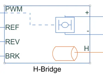
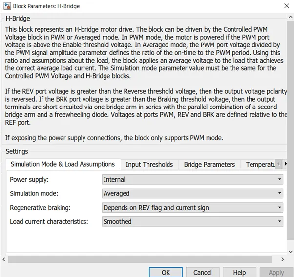
The H-Bridge block represents an H-bridge motor driver. The block has the following two Simulation mode options:
- PWM— The H-Bridge block output is a controlled voltage that depends on the input signal at the PWM If the input signal has a value greater than the Enable threshold voltage parameter value, the H-Bridge block output is on and has a value equal to the value of the Output voltage amplitude parameter. If it has a value less than the Enable threshold voltage parameter value, the block maintains the load circuit using one of the following three Freewheeling mode options:
- Via one semiconductor switch and one freewheeling diode
- Via two freewheeling diodes
- Via two semiconductor switches and one freewheeling diode
The first and third options are sometimes referred to as synchronous operation.
The signal at the REV port determines the polarity of the output. If the value of the signal at the REV port is less than the value of the Reverse threshold voltage parameter, the output has positive polarity; otherwise, it has negative polarity.
- Averaged— This mode has two Load current characteristics options:
- Smoothed
- Unsmoothed or discontinuous
The Smoothed option assumes that the current is practically continuous due to load inductance. In this case, the H-Bridge block output is:
`((V_o * V_(PWM))/A_(PWM)) – I_(out) * R_(on_`
where:
- VOis the value of the Output voltage amplitude
- VPWMis the value of the voltage at the PWM
- APWMis the value of the PWM signal amplitude
- IOUTis the value of the output current.
- RONis the Bridge on resistance
The current will be smooth if the PWM frequency is large enough. Synchronous operation where freewheeling is via a bridge arm back to the supply also helps smooth the current. For cases where the current is not smooth, or possibly discontinuous (that is, it goes to zero between PWM cycles), use the Unsmoothed or discontinuous option. For this option, you must also provide values for the Total load series resistance, Total load series inductance, and PWM frequency. During simulation, the block uses these values to calculate a more accurate value for H-bridge output voltage that achieves the same average current as would be present if simulating in PWM mode.
Set the Simulation mode parameter to Averaged to speed up simulations when driving the H-Bridge block with a Controlled PWM Voltage block. You must also set the Simulation mode parameter of the Controlled PWM Voltage block to Averaged mode. This applies the average of the demanded PWM voltage to the motor. The accuracy of the Averaged mode simulation results relies on the validity of your assumption about the load current. If you specify that the current isUnsmoothed or discontinuous, then the accuracy also depends on the values you provide for load resistance and inductance being representative. This mode also makes some simplifying assumptions about the underlying equations for the case when current is discontinuous. For typical motor and bridge parameters, accuracy should be within a few percent. To verify Averaged mode accuracy, run the simulation using the PWM mode and compare the results to those obtained from using the Averaged mode.
Braking mode is invoked when the voltage presented at the BRK port is larger than the Braking threshold voltage. Regardless of whether in PWM or Averaged mode, when in braking mode the H-bridge is modeled by a series combination of two resistances R1 and R2 where:
- R1is the resistance of a single bridge arm, that is, half the value of the Total bridge on resistance
- R2is the resistance of a single bridge arm in parallel with a diode resistance, that is, R1 Rd / ( R1 + Rd ), where Rd is the diode resistance.
Controller Specifications:-
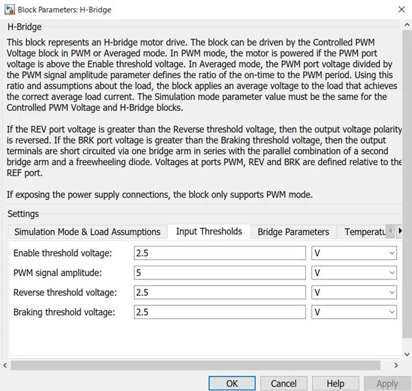
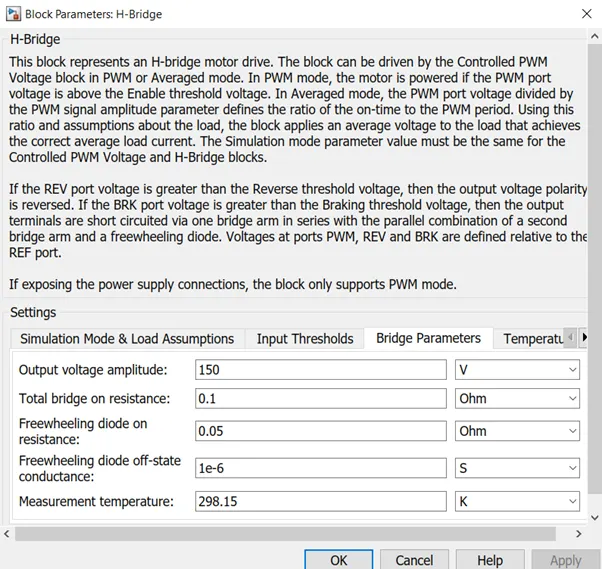
Simulation mode is set to ‘Averaged’ to set the simulation fast.
Threshold Voltage 2.5 V
PWM signal amplitude 5 V
Reverse Threshold Voltage 2.5 V
Braking Threshold Voltage 2.5 V
Output Voltage 150 V
Thermal Port
The block has an optional thermal port, hidden by default. To expose the thermal port, right-click the block in your model, and then from the context menu select Simscape > Block choices > Show thermal port. This action displays the thermal port H on the block icon, and adds the Temperature Dependence and Thermal Port parameters. These parameters are described further on this reference page.
When the thermal port is visible:
- The heat generated by the bridge on-resistance and freewheeling diodes is added to the thermal port. The thermal port has an associated thermal mass and initial temperature that you can set from the Thermal Port
- The bridge on-resistance and freewheeling diode resistance become functions of temperature. You can define the values for these resistances and the second measurement temperature from the Temperature Dependence Resistance is assumed to vary linearly between the two measurement temperatures. Extrapolation is used for temperatures outside of this range, except for when simulating in averaged mode with discontinuous load current characteristics.
DC Motor with Temperature Sensor:-
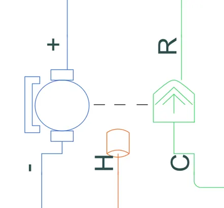
The DC Motor block represents the electrical and torque characteristics of a DC motor using the following equivalent circuit model:
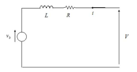
You specify the equivalent circuit parameters for this model when you set the Model parameterization parameter to By equivalent circuit parameters. The resistor R corresponds to the resistance you specify in the Armature resistance parameter. The inductor L corresponds to the inductance you specify in the Armature inductance parameter.
Thermal Port
The block has an optional thermal port, hidden by default. To expose the thermal port, right-click the block in your model, and then from the context menu select Simscape > Block choices > Show thermal port. This action displays the thermal port H on the block icon, and exposes the Temperature Dependence and Thermal Port parameters.
Use the thermal port to simulate the effects of copper resistance losses that convert electrical power to heat. For more information on using thermal ports and on the Temperature Dependence and Thermal Port parameters, see Simulating Thermal Effects in Rotational and Translational Actuators.
MOTOR Specifications:-
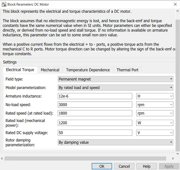
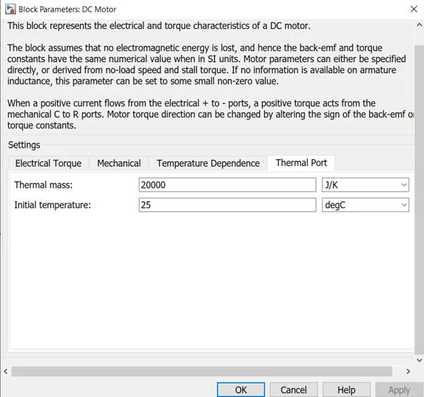
Motor parameters
No Load speed 3000 rpm
Rated speed 1800 rpm
Rated Load 1200 watts
Rated DC supply Voltage 50 V
Thermal mass 20000 J/K
Temperature sensor block:-
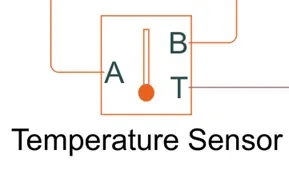
The Temperature Sensor block represents an ideal temperature sensor, that is, a device that determines the temperature differential measured between two points without drawing any heat.
Connections A and B are thermal conserving ports that connect to the two points where temperature is being monitored. Port T is a physical signal port that outputs the temperature differential value.
The block positive direction is from port A to port B. The measured temperature is determined as
`T = T_A – T_B`
Electrical Reference:-
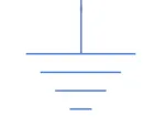
The Electrical Reference block represents an electrical ground. Electrical conserving ports of all the blocks that are directly connected to ground must be connected to an Electrical Reference block. A model with electrical elements must contain at least one Electrical Reference block.
Thermal Reference:-
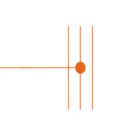
The Thermal Reference block represents a thermal reference point, that is, a point with an absolute zero temperature, with respect to which all the temperatures in the system are determined.
Rotational Reference:-
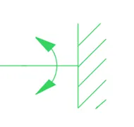
The Mechanical Rotational Reference block represents a reference point, or frame, for all mechanical rotational ports. All rotational ports that are rigidly clamped to the frame (ground) must be connected to a Mechanical Rotational Reference block
Battery Block:-
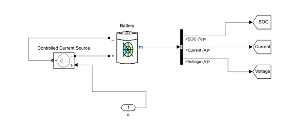
Battery specifications:-
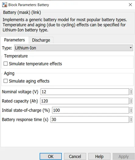
Nominal Voltage 12 V
Rated Capacity 120 Ah
SOC% 100
Response Time 30 sec
The Battery is the main Power source. Here we are using a Lithium-ion type of battery instead of Lead one. In a Lithium-ion battery, high energy density leads to low weight which translates into more kilometres between charges. While a Li-ion battery weighs 35 kg, a 48 V – 80 Ah lead acid battery weighs around 120 kg. The Controller is connected with the battery and supplies the required voltage and current as per the commands of the Driver.
Vehicle Dynamics Block:-
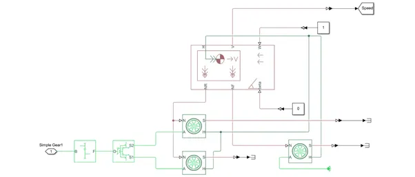
Vehicle Body:-
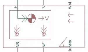
The Vehicle Body block represents a two-axle vehicle body in longitudinal motion. The vehicle can have the same or a different number of wheels on each axle. For example, two wheels on the front axle and one wheel on the rear axle. The vehicle wheels are assumed identical in size. The vehicle can also have a centre of gravity (CG) that is at or below the plane of travel.
The block accounts for body mass, aerodynamic drag, road incline, and weight distribution between axles due to acceleration and road profile. Optionally include pitch and suspension dynamics. The vehicle does not move vertically relative to the ground.
The block has an option to include an externally-defined mass and an externally-defined inertia. The mass, inertia, and centre of gravity of the vehicle body can vary over the course of simulation in response to system changes.
Vehicle specifications:-
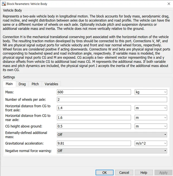
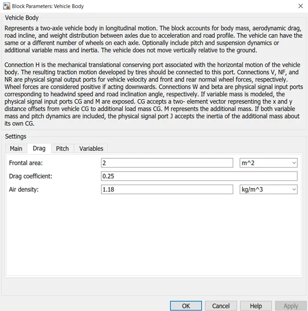
Mass of the Vehicle 600 kg
Frontal area 2 m^2
Drag coefficient 0.25
Air density 1.8 kg/m^3
Gear Block:-
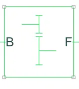
The Simple Gear block represents a gearbox that constrains the connected driveline axes of the base gear, B, and the follower gear, F, to corotate with a fixed ratio that you specify. You choose whether the follower axis rotates in the same or opposite direction as the base axis. If they rotate in the same direction, the angular velocity of the follower, ωF, and the angular velocity of the base, ωB, have the same sign. If they rotate in opposite directions, ωF and ωB have opposite signs.
The Input of the Motor will be given to the Gear block which in turn will rotate the differential of the rear wheels.
Gear specification:-
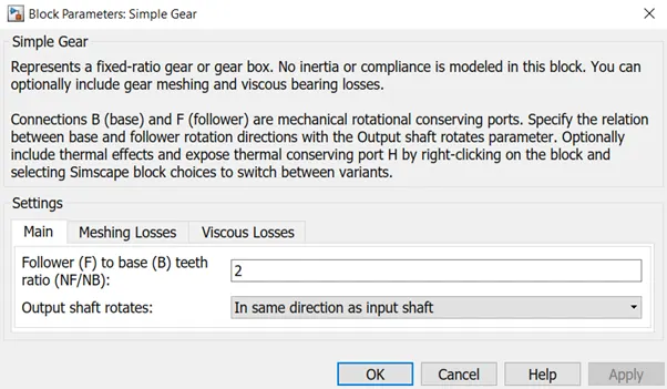
Gear ratio is set to 2 and the Direction of the output shaft is same as the direction of the input shaft in order to avoid negative velocity
Differential:-
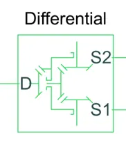
The Differential block represents a gear mechanism that allows the driven shafts to spin at different speeds. Differentials are common in automobiles, where they enable the various wheels to spin at different speeds while cornering. Ports D, S1, and S2 represent the longitudinal driving and the sun driven gear shafts of the differential. Any one of the shafts can drive the other two.
Tires:-
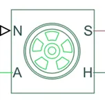
The Tire (Magic Formula) block models a tire with longitudinal behavior given by the Magic Formula [1], an empirical equation based on four fitting coefficients. The block can model tire dynamics under constant or variable pavement conditions.
The longitudinal direction of the tire is the same as its direction of motion as it rolls on pavement. This block is a structural component based on the Tire-Road Interaction (Magic Formula) block.
To increase the fidelity of the tire model, you can specify properties such as tire compliance, inertia, and rolling resistance. However, these properties increase the complexity of the tire model and can slow down simulation. Consider ignoring tire compliance and inertia if simulating the model in real time or if preparing the model for hardware-in-the-loop (HIL) simulation.
The Tire (Magic Formula) block models the tire as a rigid wheel-tire combination in contact with the road and subject to slip. When torque is applied to the wheel axle, the tire pushes on the ground (while subject to contact friction) and transfers the resulting reaction as a force back on the wheel. This action pushes the wheel forward or backward. If you include the optional tire compliance, the tire also flexibly deforms under load.
Results:-
For FTP75 Drive cycle
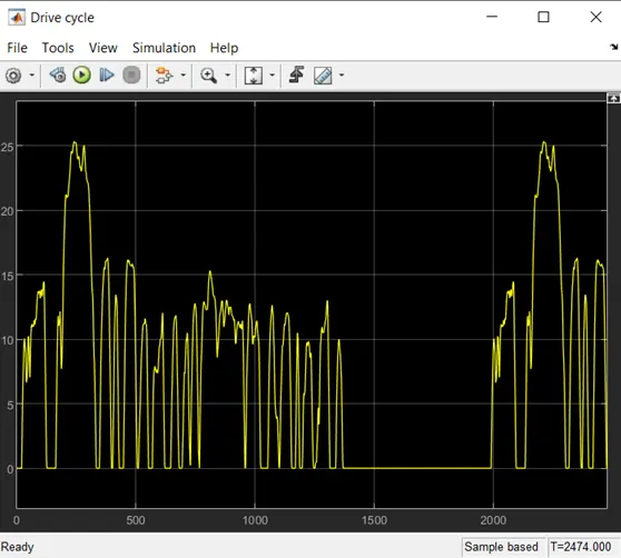
FTP75 Dive Cycle
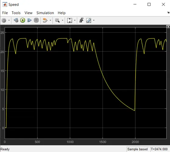
Speed
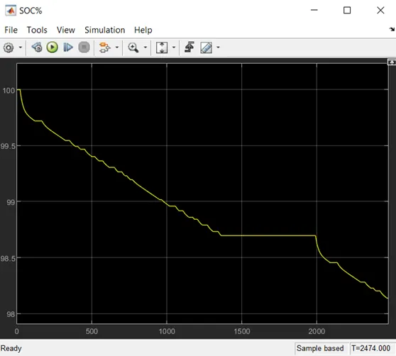
SOC%
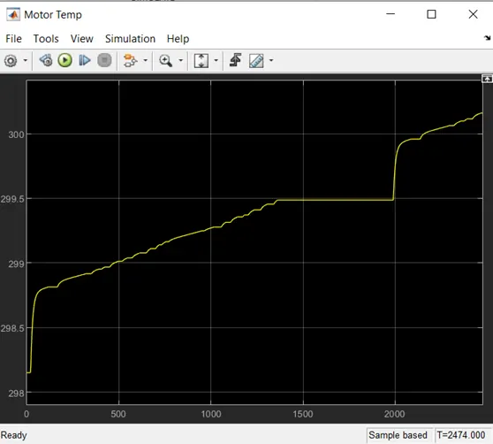
Motor Temperature
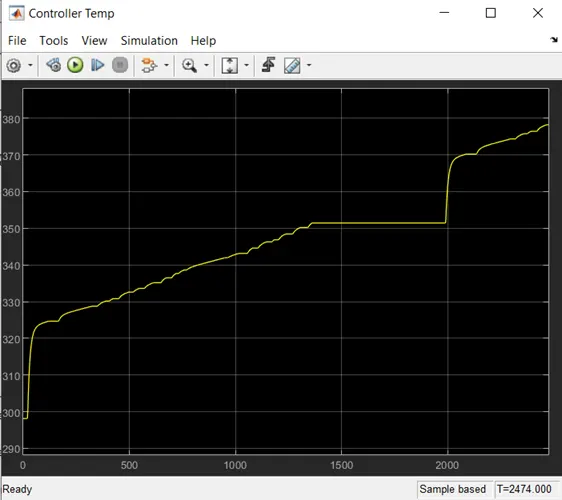
Controller Temperature
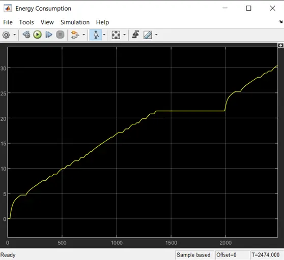
Energy Consumption
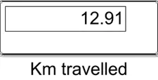
Conclusion:- Here we observe that after running the Drive cycle for 2474 seconds, the distance travelled is 12.91 km
The battery discharges to almost 98%
The motor and controller temperature goes upto 300 and 380 degrees respectively.
The energy consumption is almost 30 Wh
US06 Drive cycle:-
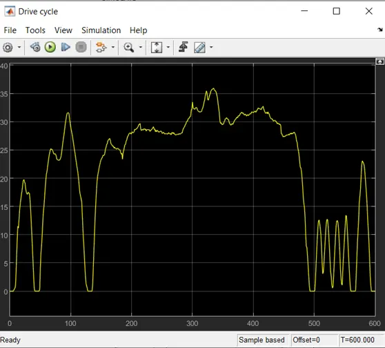
US06 Drive cycle
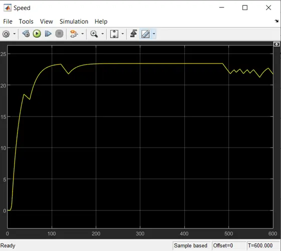
Speed
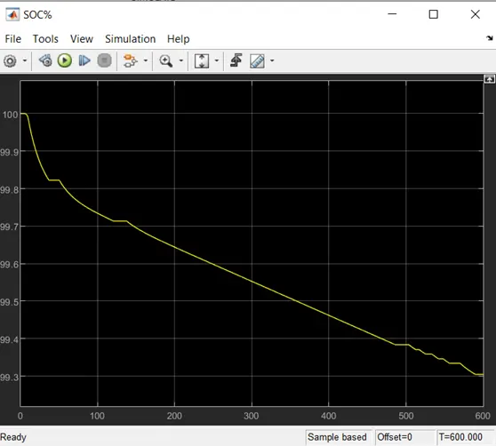
SOC%
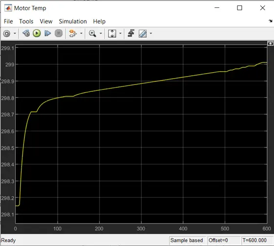
Motor Temperature
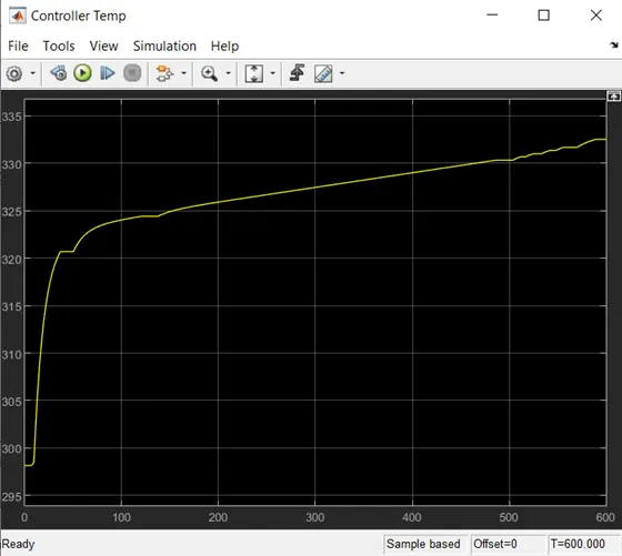
Controller Temperature
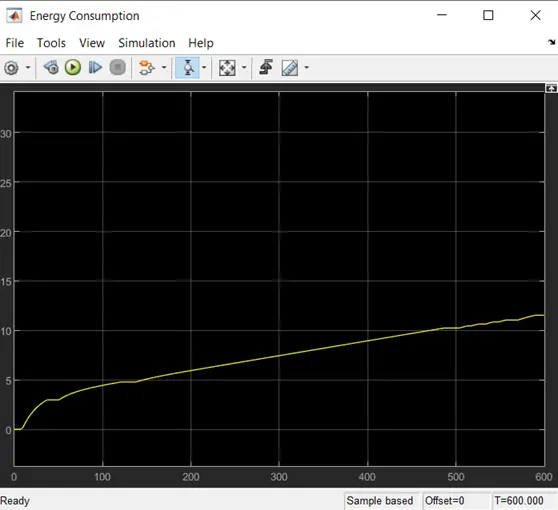
Energy Consumption
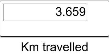
Conclusion:- Here we observe that after running the Drive cycle for 600 seconds, the distance travelled is 3.659 km
The battery discharges to almost 99.3%
The motor and controller temperature goes upto 299 and 332 degrees respectively.
The energy consumption is almost 12 Wh
SC03 Drive Cycle
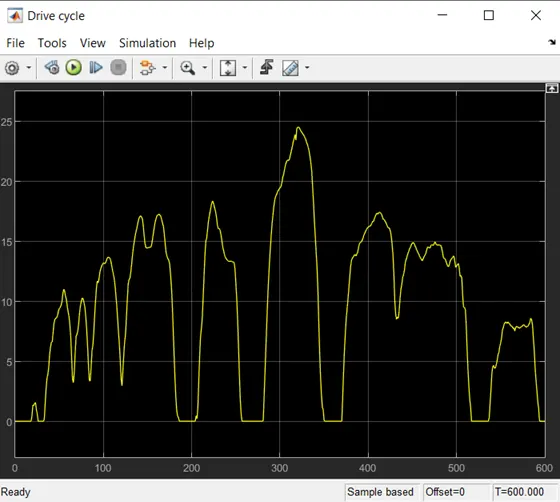
SC03 Drive Cycle
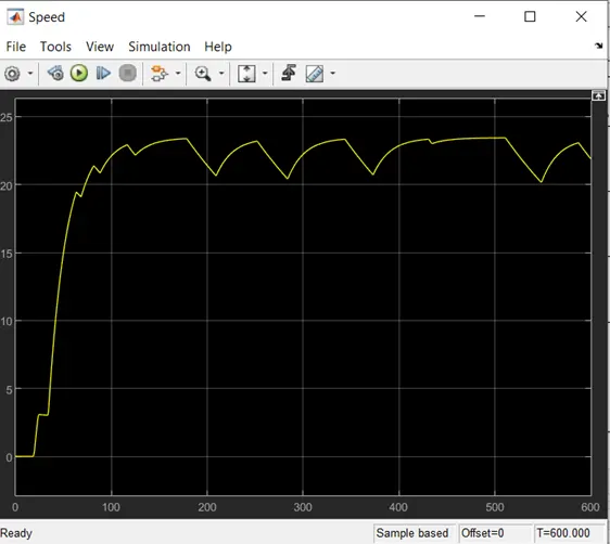
Speed
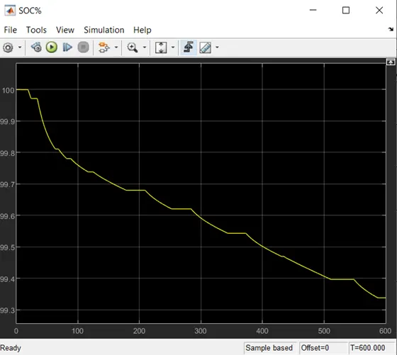
SOC%
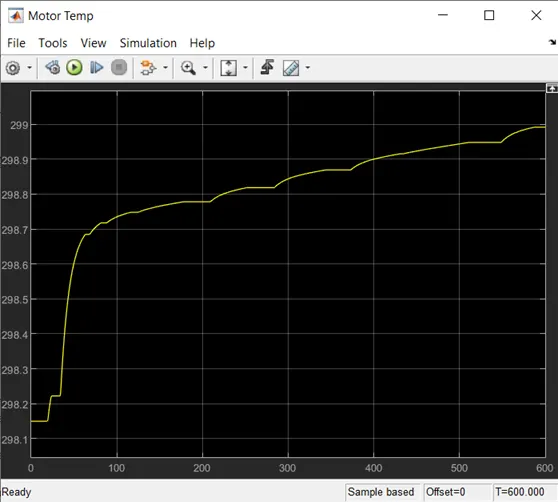
Motor Temperature
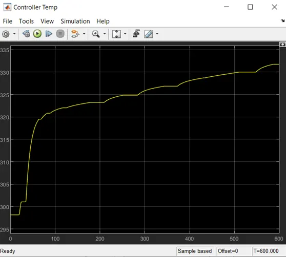
Controller Temperature
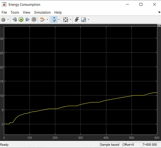
Energy consumption
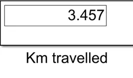
Conclusion:- Here we observe that after running the Drive cycle for 600 seconds, the distance travelled is 3.457 km
The battery discharges to almost 99.35%
The motor and controller temperature goes upto 299 and 332 degrees respectively.
The energy consumption is almost 12 Wh