Final Project: Electric Rickshaw modelling
Create a detailed MATLAB model of an electric rickshaw (three wheel passenger vehicle) as per details below:
Rear wheels driven by PM brushed type motor
Assume efficiency points of motor controller and motor
Make an excel sheet of all input and assumed data
Results: For any three standard driving cycles show energy consumption, temperature rise of motor and controller for 100 km constant speed driving at 45 kmph
Sln....
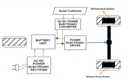
Electric rickshaws have the same principle as EV's. They also run on lithium-ion battery packs. The motors generally used here are DE motors. Mostly, electric rickshaws are rear wheel driven. The drive train is seen above. The power for the battery pack goes via an AC charger circuit with a rectifier to convert them into DC power. After charging the battery pack, the signals are sent to the electronic control unit (power converters & motor controllers). The purpose of these ECU's is to control speed according to the driver input (accelerator & brake). These pulses are then sent CO the DC motor which transfer power to the wheels.
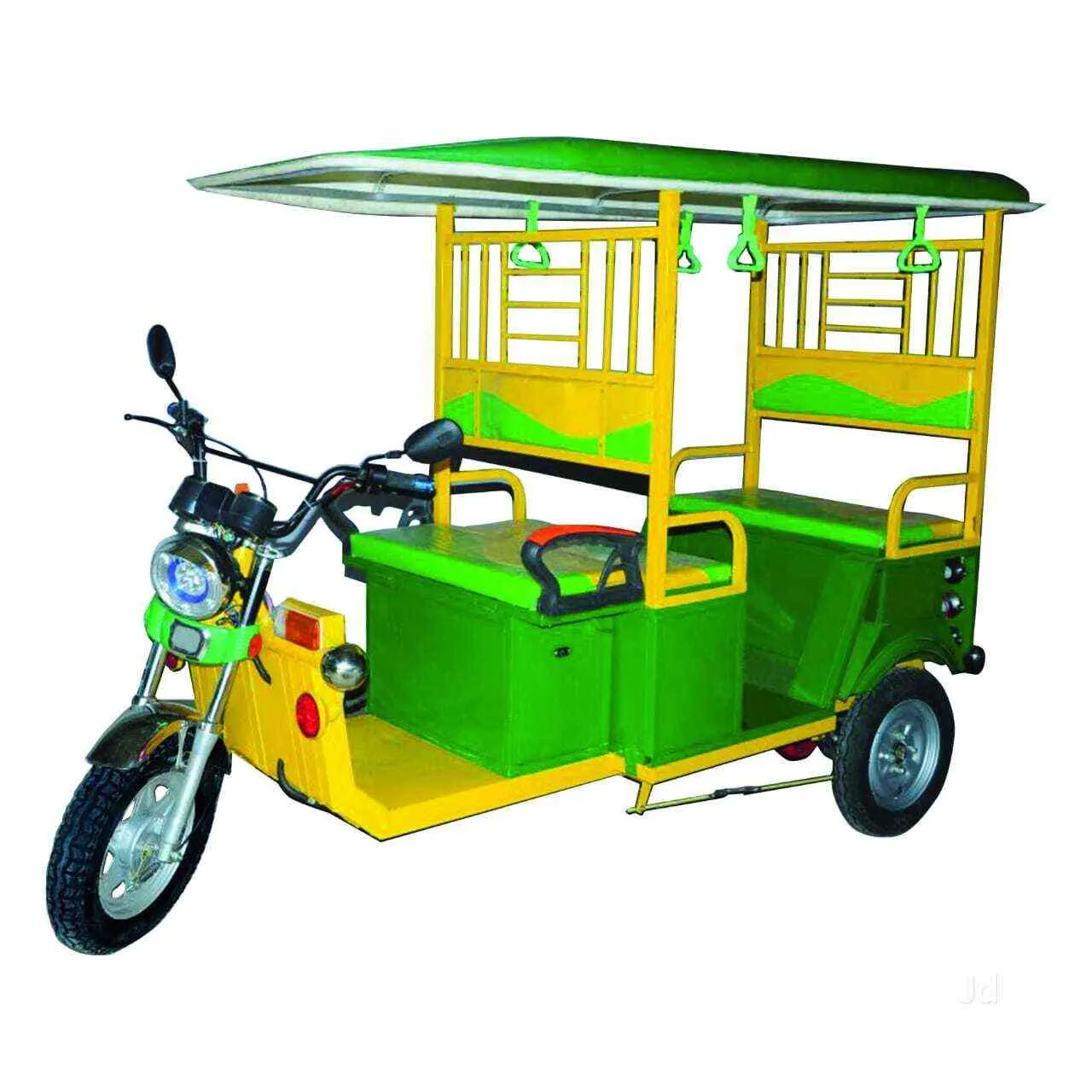
picture of an electric rickshaw is seen below.
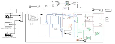
Matlab Model:
Three Different drive cycle include:
1. FTP75 drive cycle
2. WOT (User-defined)
3. UDDS drive cycle
The plot for the FTP drive cycle is shown below.
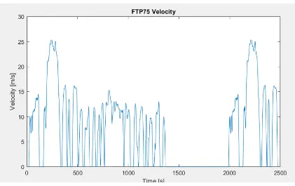
Thid drive cycle is for a time period of 2474 secs and the max velocity acheived in the drive cycle is 25m/s.
WOT (user defined)
In the question we are used to create a drive cycle for 100km at a constant speed of 45 kmph we will input them into this drive cycle
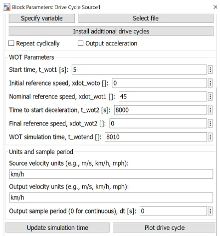
We eill calculate the drive cycle time for this WOT
Time= Distance/speed= 100/(45/3600). Since we want our drive cycle time in seconds, convert kmph into kmps)
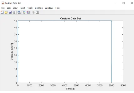
Time= 8000 Sec.
The drive cycle plot is shown below.
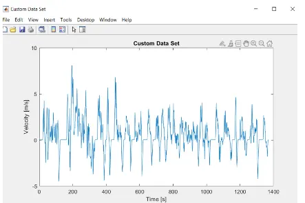
UDDS Drive cycle:
This drive cycle is called as the Urabn Dynnometer Driving Schedule. We will see the plot for this drive cycle.
Now we have selected our driving cycles. We need a block to manage these drive cycle reference during simulation This is where the multiport switch block comes into place
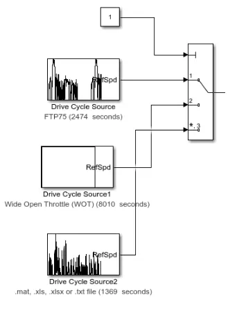
The multiport switch consists of a control port and 3 data ports as default. We can change the number of data ports for our convenience. Since there are drive cycles, we are using three data ports.
The control port is connected to a constant block. This constant block chooses the drive cycle out of the three options during run time. The FTP-75 drive cycle is numbered as 1, WOT is numbered as 2 & the UDD5 as 3.
LONGITUDINAL DRIVER:
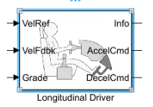
The longitudinal driver block creates a driver scenario for the system. THis block also consists of a PI controller, which is used to match the actual drive cycle of the system with the selected reference drive cycles. The parameters of the block are shown below.
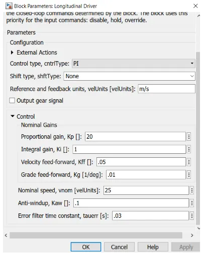
The propotional gain and integral gain are kept as default. The multiport switch output is connected to the Vel.Ref port. The Vel.Fdbk is the actual drive cycle of the system, which comes out from the vehicle body dynamics. The grade angle is kept as0.
The longitudinal driver block converts the reference drive cycle data as equivalent current & voltage signals, which are connected to the controlled voltage sources. Now we will see the motor drive system of the model.
MOTOR DRIVE:-
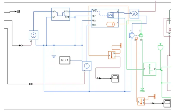
We have already decided that our motor controller would be the PWM H- bridge. This PWM H-bridge consists of 4 transistor switches with the motor at its center, making the circuit shaped as the alphabet H. These switches when open & closed, changes the direction of the current. The direction of current determines the direction in which the motor would rotate.
We nave to convert our controlled voltages into controlled PWM voltages. This is done with the help of the controlled PW voltage block, which changes the pulse width of the signals according to the controller requirement.
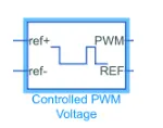
They are passed on to the controller. The controller parameters are shown below. The controlled PWM voltage block converts the voltage signals to the parameters shown below.
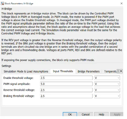
The enable threshold voltage, reverse threshold & braking threshold are kept at 2.5V. These parameters are the limit at which the motor starts to enable( switch on), stop and reverse the motor. If the voltage at REV, BRK & PWM are greater than the threshold voltage, the motor activates the braking, reverse conditions. The signal amplitude is kept high at 5V.
the output voltage of the H-bridge is kept at 330V, same cit as theoperating voltage of the motor.
We add a thermal port to the H-bridge, because we are asked tomonitor the thermal effects of the controller during simulation. This will give us an idea of what temperature the controller is during driving. Use the temperature sensor block, the thermal reference and the scope window to get the temperature plot. Now the controller is connected to the DC motor. The parameters of the DC motor are seen below.
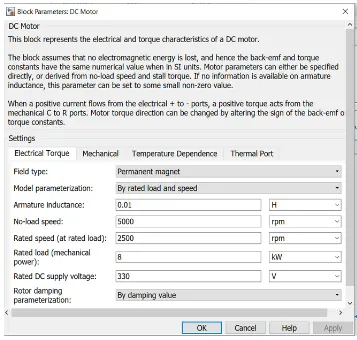
The motor parameters are entered as per the specifications given in the spreadsheet. We also add a thermal port to the DC motor to track its temperature at various speeds. Use the temperature sensor block, the thermal reference and the scope window to get the temperature plot. Now that the motor drive is finished, we will look at the vehicle body dynamics of the electric rickshaw.
VEHICLE BODY DYNAMICS:-
we will look at the block diagram of the vehicle body.
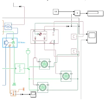
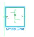
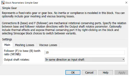
The Dc motor is connected to the simple gear block which is used to transfer the power to the wheels of the vehicle The Parameters of the simple gear block is shown below.
Tyres of the Vehicle
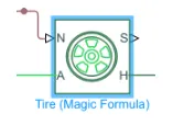
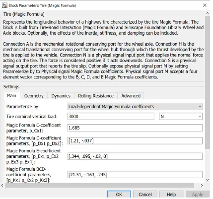
Its Parameters Shown below.
The Rolling Resistance is enabled and the parameters are shown below.
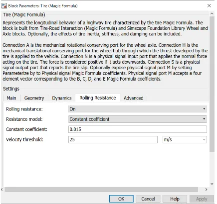
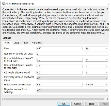
Now we will look into the vehicle body parameters. Use the vehicle body dynamics block to simulate a vehicle body based on the weight, centre of gravity, frontal area & drag co-efficient.
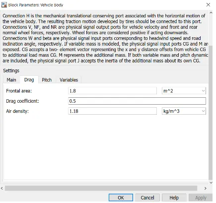
The Frontal area & the drag co efficient are also enabled.
Connect the tire blocks to the vehicle body as shown in the model screenshot. We have not considered the grade angle & the wind velocity for the electric rickshaw. Hence the values are to be specified as zero. Use the PS constant block to specify the values to the vehicle body.
Create a display block to display the speed of the vehicle in Kmph. Since our drive cycle data are in m/s, multiply the output velocity by 3.6 to get the values in kmph.
The output velocity is fedback to the longitudinal driver block. The reference and the actual drive cycle data is attached to a scope window to compare the results. Now we will see the battery system of the electric rickshaw.
BATTERY SYSTEM:-
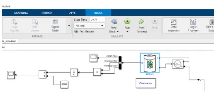
A current sensor is connected to the 1-bridge controller & the signals are sent to a controlled current source.
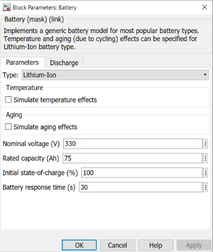
Then the generic battery block is connected across it. The battery parameters are entered aIS oer the pack specifications.