Final Project: Electric Rickshaw modelling

AIM:

Create a detailed MATLAB model of an electric rickshaw (three-wheel passenger vehicle) as per the details below:

Rear wheels driven by PM brushed type motor

1. Assume efficiency points of motor controller and motor, Make an excel sheet of all input and assumed data
2. Results: For any three standard driving cycles show energy consumption, the temperature rise of the motor and controller for 100 km constant speed driving at 45 mph.

(Note- The Simulink model file should be compulsorily attached)

Explanation:

MATLAB model of an electric rickshaw:

Settings for 100 km constant speed driving at 45 mph:

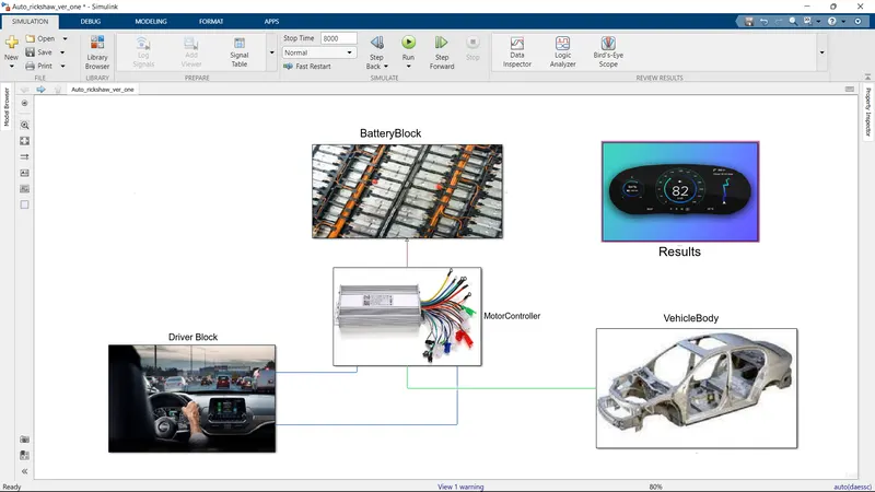
Driver Block:

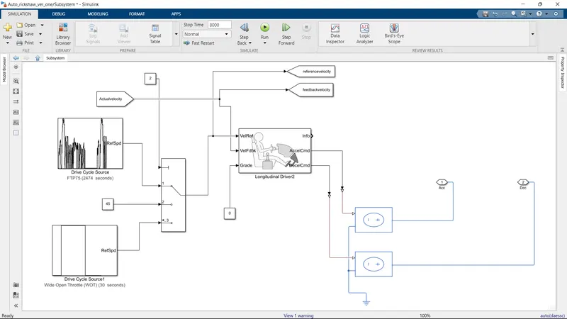
Longitudinal Block:

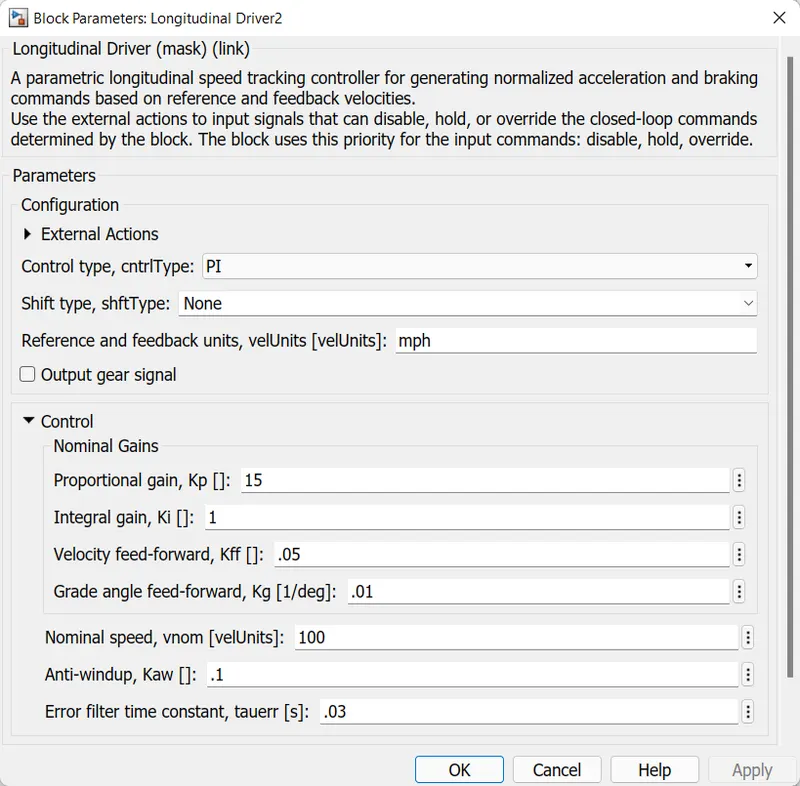
WOT :

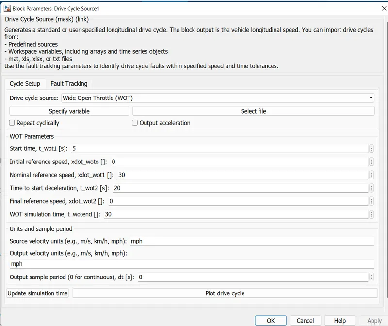
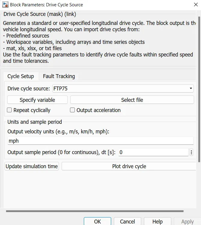
Drive Cycle FTP24:

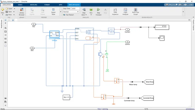
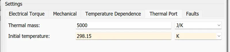
Motor Controller Block:

Controlled PWM voltage:

1. The output from the longitudinal driver both Acceleration and deceleration commands are given to the motor controller block.

2. Acceleration command is given to +ref port of controlled PWM voltage block whereas the deceleration command is given to H bridge brake port.

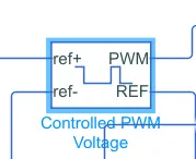
This block creates a Pulse-Width Modulated (PWM) voltage across the PWM and REF ports. The output voltage is zero when the pulse is low, and is equal to the Output voltage amplitude parameter when high. Duty cycle is set by the input value. Right-click the block and select Simscape->Block choices to switch between electrical +ref/-ref ports and PS input u to specify the input value.

At time zero, the pulse is initialized as high unless the duty cycle is set to zero or the Pulse delay time is greater than zero.

The Simulation mode can be set to PWM or Averaged. In PWM mode, the output is a PWM signal. In Averaged mode, the output is constant with value equal to the averaged PWM signal.

Settings:

PWM frequency: 1000 Hz

Simulation mode: Averaged

input Scaling:

Input voltage for 0% duty cycle : 0

Input voltage for 100% duty cycle : 1

Output Voltage:

Output voltage amplitude: 5V

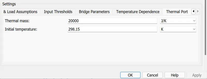
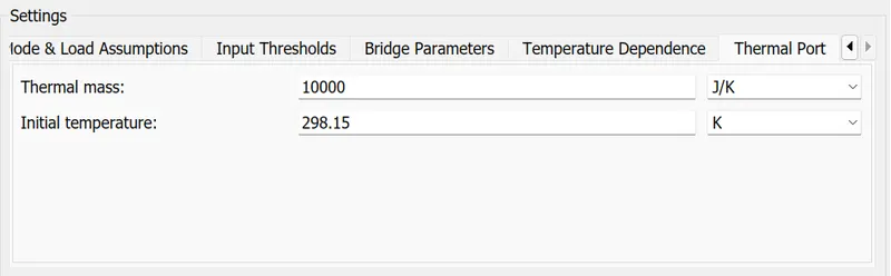
H-Bridge with Thermal Port:

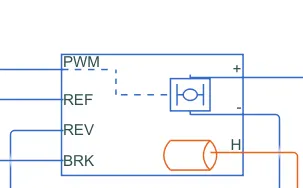
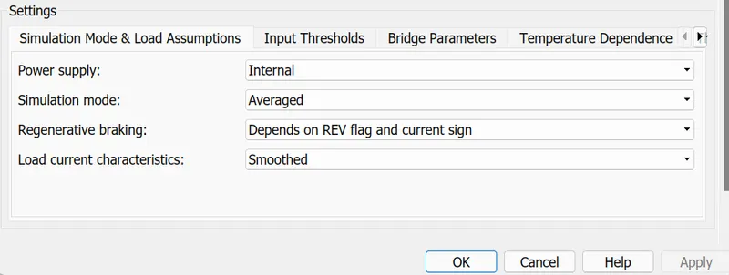
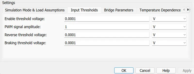
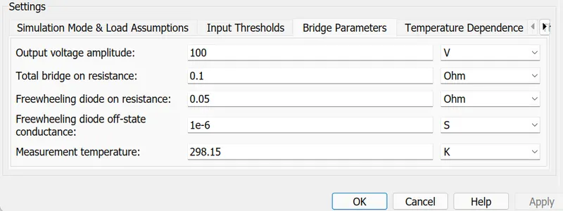
This block represents an H-bridge motor drive. The block can be driven by the Controlled PWM Voltage block in PWM or Averaged mode. In PWM mode, the motor is powered if the PWM port voltage is above the Enable threshold voltage. In Averaged mode, the PWM port voltage divided by the PWM signal amplitude parameter defines the ratio of the on-time to the PWM period. Using this ratio and assumptions about the load, the block applies an average voltage to the load that achieves the correct average load current. The Simulation mode parameter value must be the same for the Controlled PWM Voltage and H-Bridge blocks.

If the REV port voltage is greater than the Reverse threshold voltage, then the output voltage polarity is reversed. If the BRK port voltage is greater than the Braking threshold voltage, then the output terminals are short circuited via one bridge arm in series with the parallel combination of a second bridge arm and a freewheeling diode. Voltages at ports PWM, REV and BRK are defined relative to the REF port.

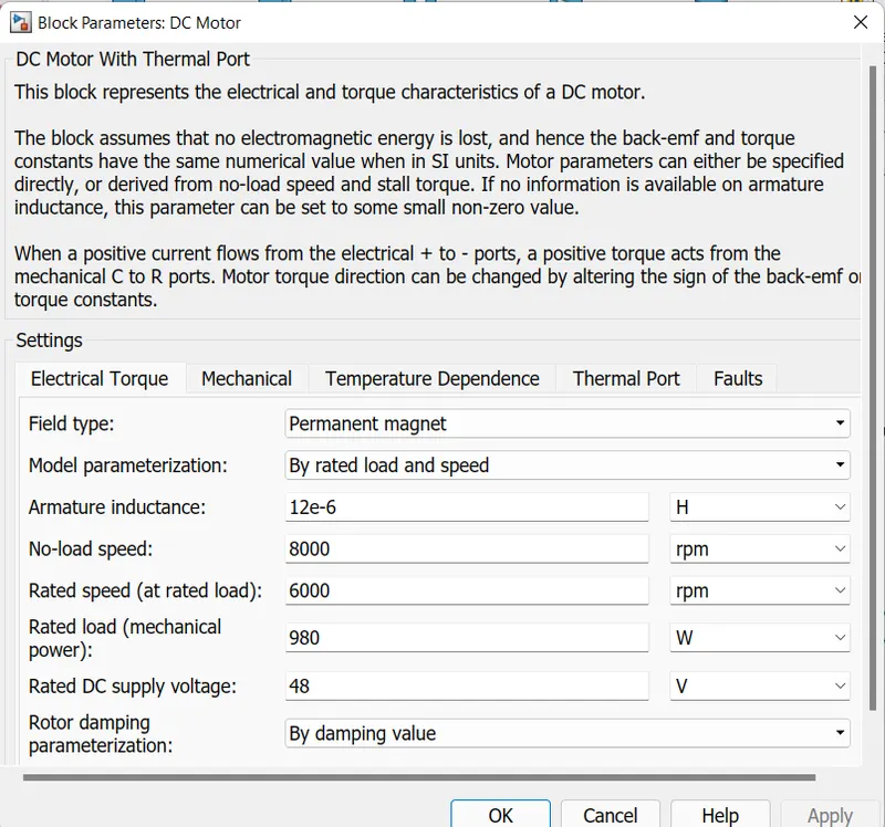
DC motor with Thermal Port:

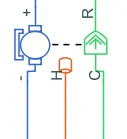
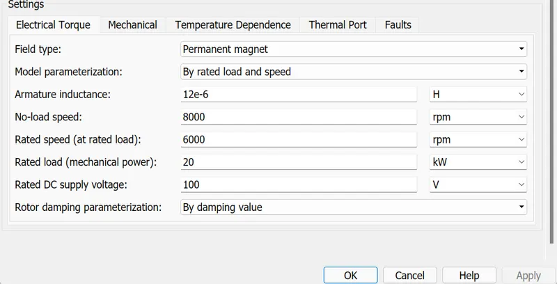
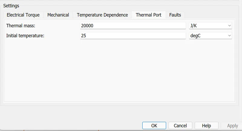
This block represents the electrical and torque characteristics of a DC motor.

The block assumes that no electromagnetic energy is lost, and hence the back-emf and torque constants have the same numerical value when in SI units. Motor parameters can either be specified directly or derived from the no-load speed and stall torque. If no information is available on armature inductance, this parameter can be set to some small non-zero value.

When a positive current flows from the electrical + to - ports, a positive torque acts from the mechanical C to R ports. Motor torque direction can be changed by altering the sign of the back-emf or torque constants.

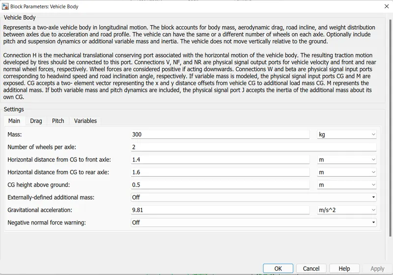
Vehicle Body:

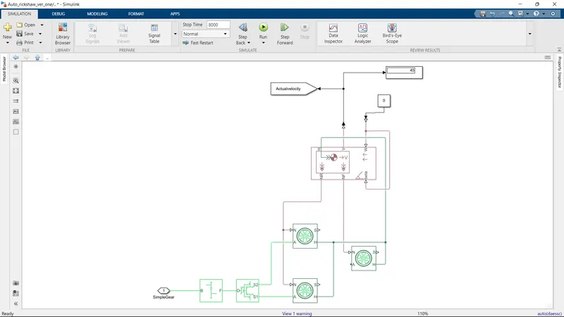
Vehicle Body Block:

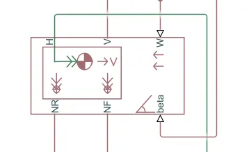
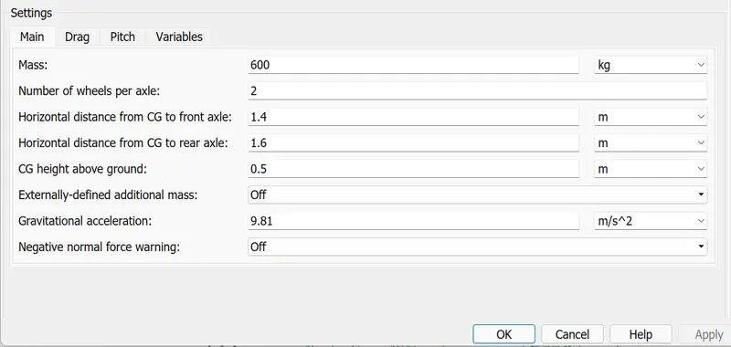
Represents a two-axle vehicle body in longitudinal motion. The block accounts for body mass, aerodynamic drag, road incline, and weight distribution between axles due to acceleration and road profile. The vehicle can have the same or a different number of wheels on each axle. Optionally include pitch and suspension dynamics or additional variable mass and inertia. The vehicle does not move vertically relative to the ground.

Connection H is the mechanical translational conserving port associated with the horizontal motion of the vehicle body. The resulting traction motion developed by tires should be connected to this port. Connections V, NF, and NR are physical signal output ports for vehicle velocity and front and rear normal wheel forces, respectively. Wheel forces are considered positive if acting downwards. Connections W and beta are physical signal input ports corresponding to headwind speed and road inclination angle, respectively. If variable mass is modeled, the physical signal input ports CG and M are exposed. CG accepts a two- element vector representing the x and y distance offsets from vehicle CG to additional load mass CG. M represents the additional mass. If both variable mass and pitch dynamics are included, the physical signal port J accepts the inertia of the additional mass about its own CG.

Tire Magic formula:

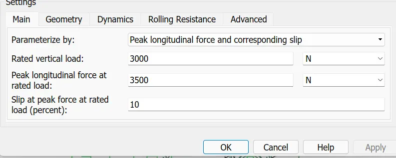
Represents the longitudinal behavior of a highway tire characterized by the tire Magic Formula. The block is built from Tire-Road Interaction (Magic Formula) and Simscape Foundation Library Wheel and Axle blocks. Optionally, the effects of tire inertia, stiffness, and damping can be included.

Connection A is the mechanical rotational conserving port for the wheel axle. Connection H is the mechanical translational conserving port for the wheel hub through which the thrust developed by the tire is applied to the vehicle. Connection N is a physical signal input port that applies the normal force acting on the tire. The force is considered positive if it acts downwards. Connection S is a physical signal output port that reports the tire slip. Optionally expose physical signal port M by setting Parameterize by to Physical signal Magic Formula coefficients. Physical signal port M accepts a four-element vector corresponding to the B, C, D, and E Magic Formula coefficients.

Simple gear:

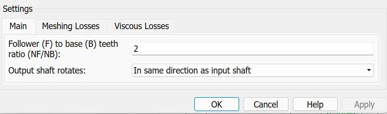
Represents a fixed-ratio gear or gear box. No inertia or compliance is modeled in this block. You can optionally include gear meshing and viscous bearing losses.

Connections B (base) and F (follower) are mechanical rotational conserving ports. Specify the relation between base and follower rotation directions with the Output shaft rotates parameter. Optionally include thermal effects and expose thermal conserving port H by setting Friction model to a temperature-dependent setting.

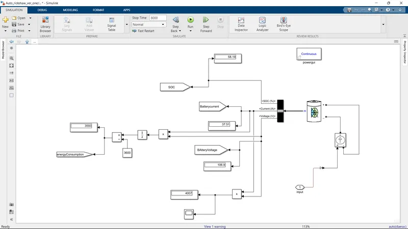
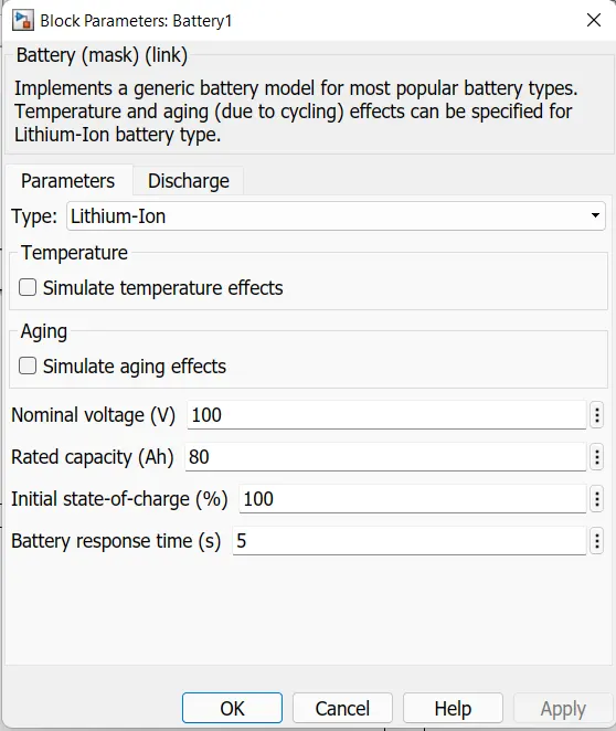
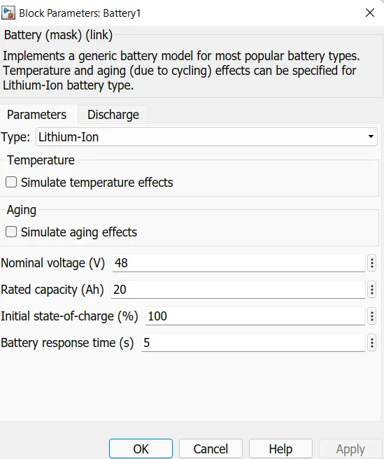
Battery Block:

Results:

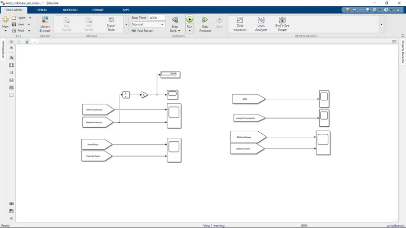
Reference velocity Vs Actual Velocity:

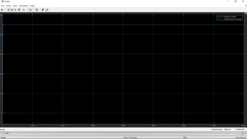
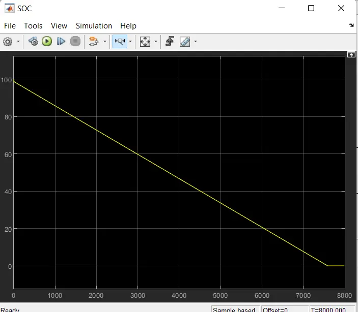
State of Charge:

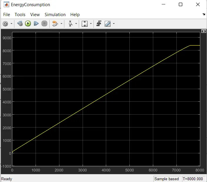
Energy Consumption:

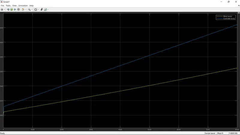
Motor Temperature and controller temperature:

Settings for FTP24:

H-Bridge settings:

Battery Settings:

Vehicle Body settings:

Results:

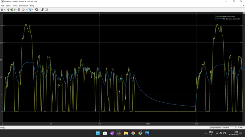
Reference velocity Vs Actual Velocity:

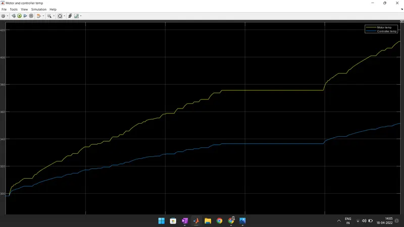
Motor and Motor controller temperature:

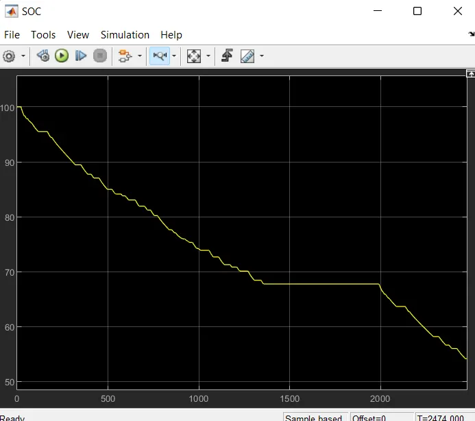
SOC:

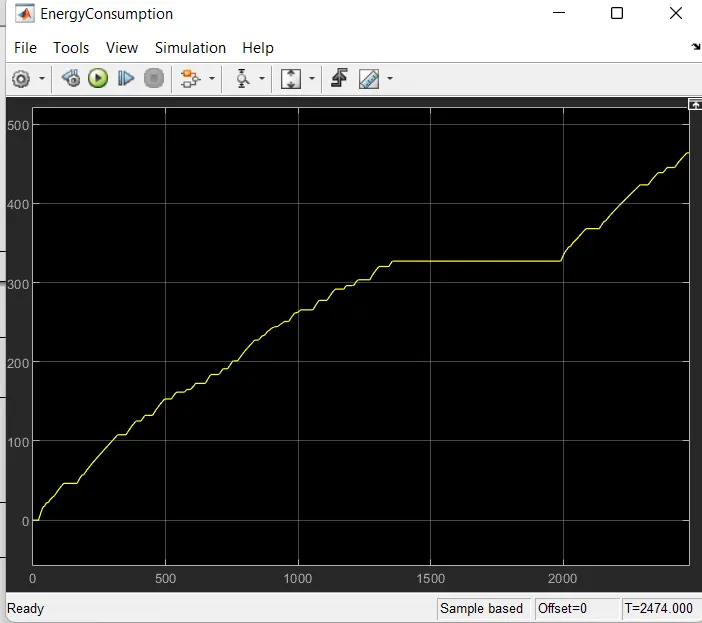
EnergyConsumption:

UDDS drive cycle Condition results:

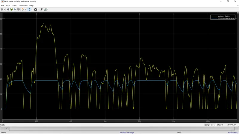
Reference velocity Vs Actual Velocity:

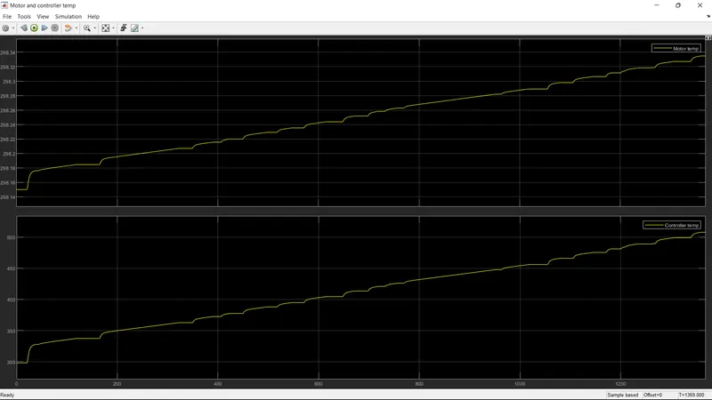
Motor and Motor controller temperature:

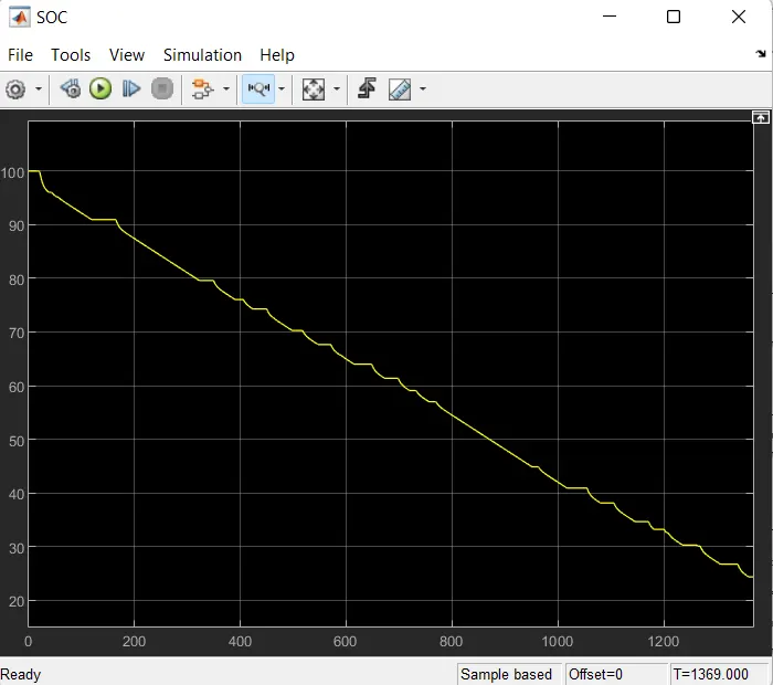
SOC:

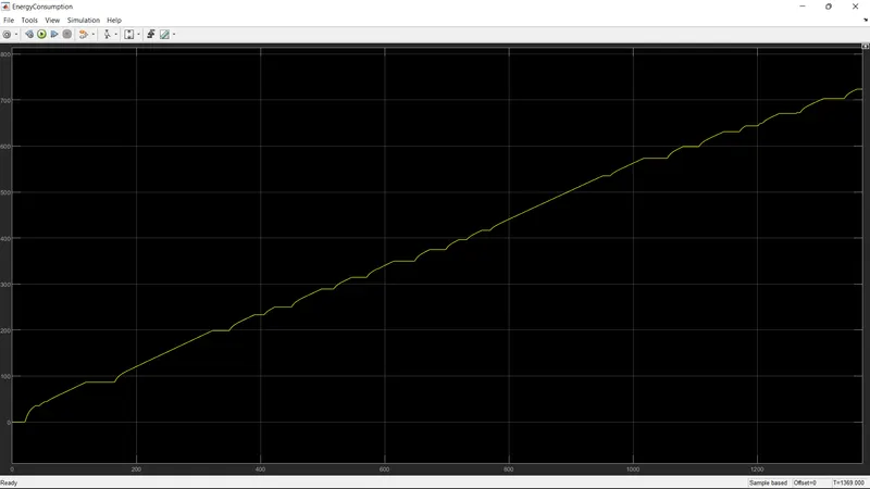
Energy Consumption:

Conclusion:

1. The vehicle has run a distance of 100Kms at 45mph speed with no state of charge, assumed values and the Model has been attached.