Week 4.1 - Genetic Algorithm

Aim : To optimise the given stalagmite function and Find the global maxima.

Code:

close all
clear all
clc

% search space
x = linspace(0,1,200);
y = linspace(0,1,200);
num_cases = 50;

% Creating 2d mesh
[xx yy] = meshgrid(x, y);

% Evaluating the stalagmite function
for i = 1 : length(xx)
    for j = 1 : length(yy)
        input(1) = xx(i,j);
        input(2) = yy(i,j);
        f(i,j) = stalagmite(input);
    end
end

% study1 : Statistical beheviour - Unbounded inputs
tic
for k = 1 : num_cases
    [input1 Fopt1(k)] = ga(@stalagmite, 2);
    Xopt1(k) = input1(1);
    Yopt1(k) = input1(2);
end

Time1 = toc
Fopt1 = -Fopt1;
f = -f;


% Plotting
figure(1)

subplot(2,1,1)
hold on
surfc(xx, yy, f)
shading interp
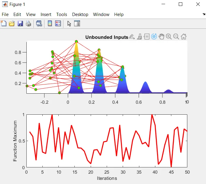
plot3(Xopt1, Yopt1, Fopt1, 'color', 'r', 'marker', 'o', 'markersize' ,5 ,'markerfacecolor', 'g')
title('Unbounded Inputs')


subplot(2,1,2)
plot(Fopt1, 'color', 'r', 'linewidth', 2)
xlabel('Iterations')
ylabel('Function Maximum')


% study2 : Statistical beheviour - Bounded Inputs

tic
for k = 1 : num_cases
    [input2 Fopt2(k)] = ga(@stalagmite, 2, [], [], [], [], [0;0], [1;1]);
    Xopt2(k) = input2(1);
    Yopt2(k) = input2(2);
end

Time2 = toc
Fopt2 = -Fopt2;

% Plotting
figure(2)

subplot(2,1,1)
hold on
surfc(xx, yy, f)
shading interp
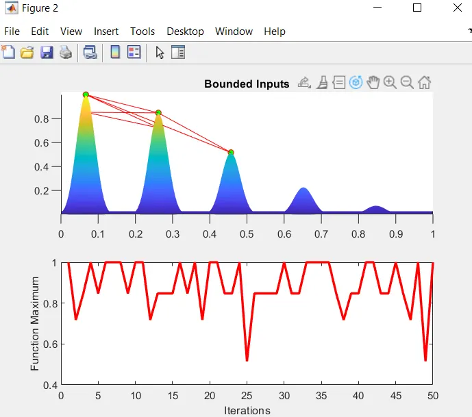
plot3(Xopt2, Yopt2, Fopt2, 'color', 'r', 'marker', 'o', 'markersize' ,5 ,'markerfacecolor', 'g')
title('Bounded Inputs')

subplot(2,1,2)
plot(Fopt2, 'color', 'r', 'linewidth', 2)
xlabel('Iterations')
ylabel('Function Maximum')


% study3 : Statistical behaviour - Bounded Inputs with modified population

options = optimoptions('ga');
options = optimoptions(options, 'PopulationSize', 200);

tic
for k = 1 : num_cases
    [input3 Fopt3(k)] = ga(@stalagmite, 2, [], [], [], [], [0;0], [1;1], [], [], options);
    Xopt3(k) = input3(1);
    Yopt3(k) = input3(2);
end

Time3 = toc
Fopt3 = -Fopt3;

% Plotting
figure(3)

subplot(2,1,1)
hold on
surfc(xx, yy, f)
shading interp
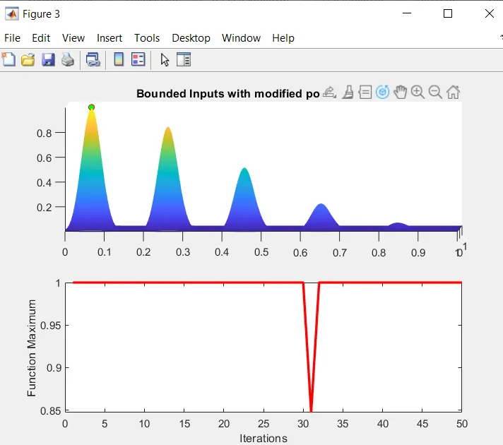
plot3(Xopt3, Yopt3, Fopt3, 'color', 'r', 'marker', 'o', 'markersize' ,5 ,'markerfacecolor', 'g')
title('Bounded Inputs with modified population size')


subplot(2,1,2)
plot(Fopt3, 'color', 'r', 'linewidth', 2)
xlabel('Iterations')
ylabel('Function Maximum')

% rng = random number ganerator set to default
% To reproduce random numbers generated in first run, to get same results
% in whenever code is run
rng('default');
 

stalagmite function:

% Stalagmite Function
function f = stalagmite(input)

x = input(1);
y = input(2);
f1x = (sin((5.1*pi)*x + 0.5))^6;
f1y = (sin((5.1*pi)*y + 0.5))^6;
f2x = exp((-4*log(2))*((x-0.0667)^2)/0.64);
f2y = exp((-4*log(2))*((y-0.0667)^2)/0.64);

f = -f1x*f2x*f1y*f2y;   % -ve sign for finding maximum value
end

Results for all the Three cases :

Case1: Ubbounded Inputs

Case 2: Bounded Inputs

Case3 : Bounded inputs with Modified Population

Genetic Algorithm : its an algorithm which uses evolution technique,here all the population members are assigned with a fitness value which is used to select the parents for next generation.Children can be generated using some techniques like mutations or combinations ,ince children are generated then they replace old population and form as new generation.

Syntax for GA:

1. x = ga(Fun,nvars) finds a local unconstrained minimum, x, to the objective function, Fun. nvars is the dimension (number of design variables) of fun.

2. X= ga(Fun,nvras,A,B) finds a local minimum x to fun, subject to the linear inequalities A*x ≤ b. ga evaluates the matrix product A*x as if x is transposed (A*x').

3. x = ga(fun,nvars,A,b,Aeq,beq) finds a local minimum x to fun, subject to the linear equalities Aeq*x = beq and A*x ≤ b. (Set A=[] and b=[] if no linear inequalities exist.) ga evaluates the matrix product Aeq*x as if x is transposed (Aeq*x').

4.x = ga(fun,nvars,A,b,Aeq,beq,lb,ub) defines a set of lower and upper bounds on the design variables, x, so that a solution is found in the range lb ≤ x ≤ ub. (Set Aeq=[] and beq=[] if no linear equalities exist.)

5.x = ga(fun,nvars,A,b,Aeq,beq,lb,ub,nonlcon) subjects the minimization to the constraints defined in nonlcon. The function nonlcon accepts x and returns vectors C and Ceq, representing the nonlinear inequalities and equalities respectively. ga minimizes the fun such that C(x) ≤ 0 and Ceq(x) = 0. (Set lb=[] and ub=[] if no bounds exist.)

6.x = ga(fun,nvars,A,b,Aeq,beq,lb,ub,nonlcon,options) minimizes with the default optimization parameters replaced by values in options. (Set nonlcon=[] if no nonlinear constraints exist.) Create options using optimoptions.

7.x = ga(fun,nvars,A,b,Aeq,beq,lb,ub,nonlcon,intcon) or x = ga(fun,nvars,A,b,Aeq,beq,lb,ub,nonlcon,intcon,options) requires that the variables listed in intcon take integer values.

8.x = ga(problem) finds the minimum for problem, a structure described in problem.

9.[x,fval] = ga(___), for any previous input arguments, also returns fval, the value of the fitness function at x.