Final Project: Electric Rickshaw modelling

Create a detailed MATLAB model of an electric rickshaw (three wheel passenger vehicle) as per details below:

Rear wheels driven by PM brushed type motor

Assume efficiency points of motor controller and motor

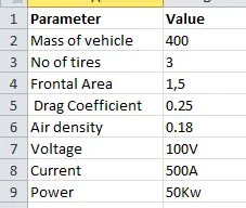
Make an excel sheet of all input and assumed data

Results: For any three standard driving cycles show energy consumption, temperature rise of motor and controller for 100 km constant speed driving at 45 kmph.

Aim of the project.

The aim of the project is to

-familarise with electric vehicle modeling.

-Observe the hermal change in vehicle electrical components and motor.

-Observe the relationship between motor control, battery and drive cycle.

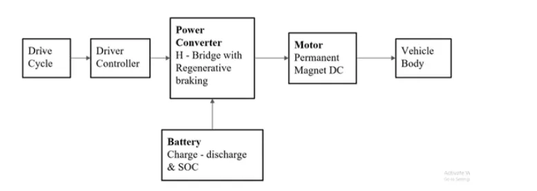
Block diagram of the simulation.

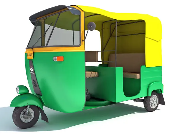
-The vehicle to be modeled is a simple an electric rickshaw (three wheel passenger vehicle)

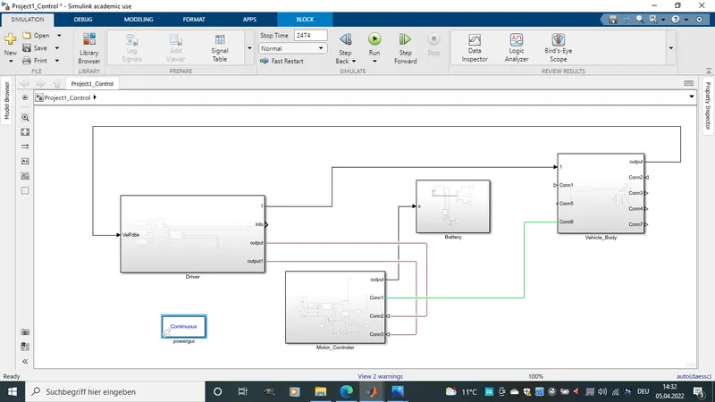
Vehicle Model:

Vehicle Body Subsystem.

This subsystem comprises of vehicle body block, tires and gear. It summarises the body framework of a vehicle including its tires, Axel , suspentions and gearbox. The blocks making up this subsystem are explained below.

Vehicle body:

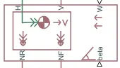
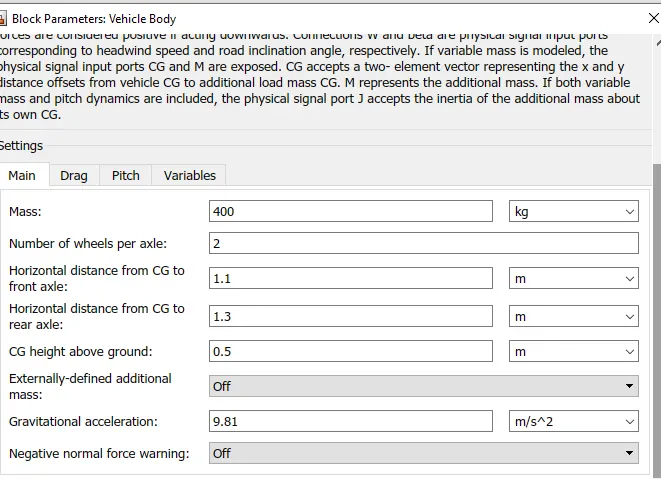
The Vehicle Body block represents a two-axle vehicle body in longitudinal motion. The vehicle can have the same or a different number of wheels on each axle. For example, two wheels on the front axle and one wheel on the rear axle. The vehicle wheels are assumed identical in size. The vehicle can also have a center of gravity (CG) that is at or below the plane of travel.

The block accounts for body mass, aerodynamic drag, road incline, and weight distribution between axles due to acceleration and road profile. Optionally include pitch and suspension dynamics. The vehicle does not move vertically relative to the ground.

The block has an option to include an externally-defined mass and an externally-defined inertia. The mass, inertia, and center of gravity of the vehicle body can vary over the course of simulation in response to system changes.

Tire (Magic formula):

The Tire (Magic Formula) block models a tire with longitudinal behavior given by the Magic Formula [1], an empirical equation based on four fitting coefficients. The block can model tire dynamics under constant or variable pavement conditions.

The longitudinal direction of the tire is the same as its direction of motion as it rolls on pavement. This block is a structural component based on the Tire-Road Interaction(Magic Formula) block.

To increase the fidelity of the tire model, you can specify properties such as tire compliance, inertia, and rolling resistance. However, these properties increase the complexity of the tire model and can slow down simulation. Consider ignoring tire compliance and inertia if simulating the model in real time or if preparing the model for hardware-in-the-loop (HIL) simulation.

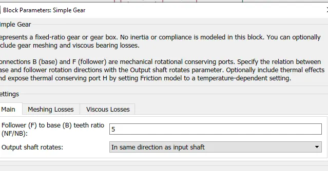
Simple Gear and Differential:

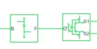
The Simple Gear block represents a gearbox that constrains the connected driveline axes of the base gear, B, and the follower gear, F, to corotate with a fixed ratio that you specify. You choose whether the follower axis rotates in the same or opposite direction as the base axis. If they rotate in the same direction, the angular velocity of the follower, ω_F, and the angular velocity of the base, ω_B, have the same sign. If they rotate in opposite directions, ω_F and ω_B have opposite signs.

Motor Control Subsystem.

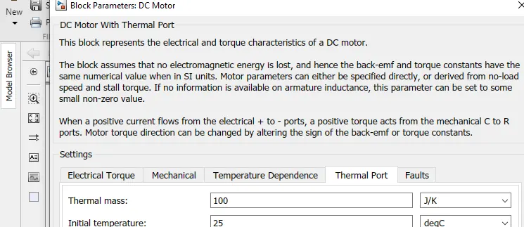
In this subsystem a DC motor , H-bridge controler and a PWM are conected to provide the motor with the appropriate voltage to produce the required speed. A temperature sensor is connected to both the motor and its controler to evaluate the heat dissipated during the drive.

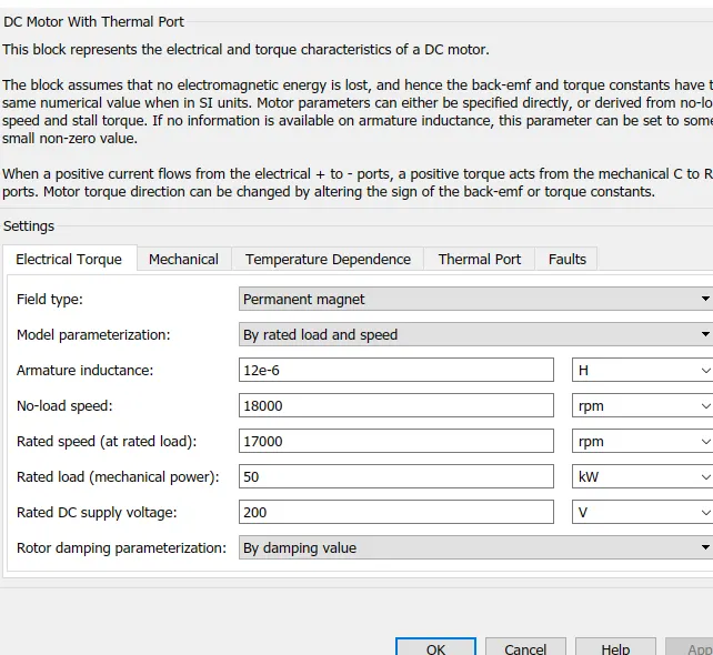
DC Motor:

The DC Motor block represents the electrical and torque characteristics of a DC motor using the following equivalent circuit model:

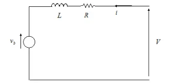
You specify the equivalent circuit parameters for this model when you set the Model parameterization parameter to By equivalent circuit parameters. The resistor R corresponds to the resistance you specify in the Armature resistance parameter. The inductor L corresponds to the inductance you specify in the Armature inductance parameter.

You can specify how to generate the magnetic field of the DC motor by setting the Field type parameter to the desired option. The permanent magnets in the motor induce the following back emf v_b in the armature:

H-Bridge:

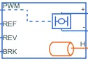
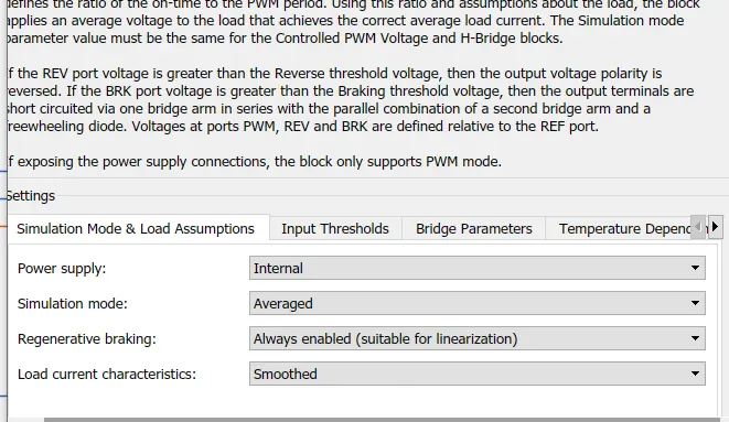
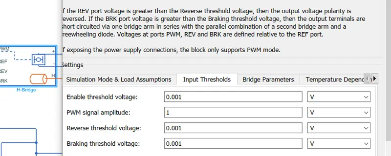
PWM — The H-Bridge block output is a controlled voltage that depends on the input signal at the PWM port. If the input signal has a value greater than the Enable threshold voltage parameter value, the H-Bridge block output is on and has a value equal to the value of the Output voltage amplitude parameter. If it has a value less than the Enable threshold voltage parameter value, the block maintains the load circuit using one of the following three Freewheeling mode options:

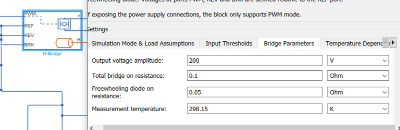
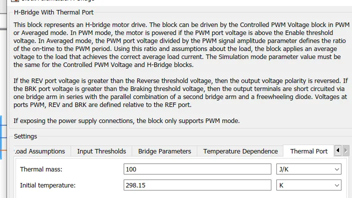
Driver Subsystem.

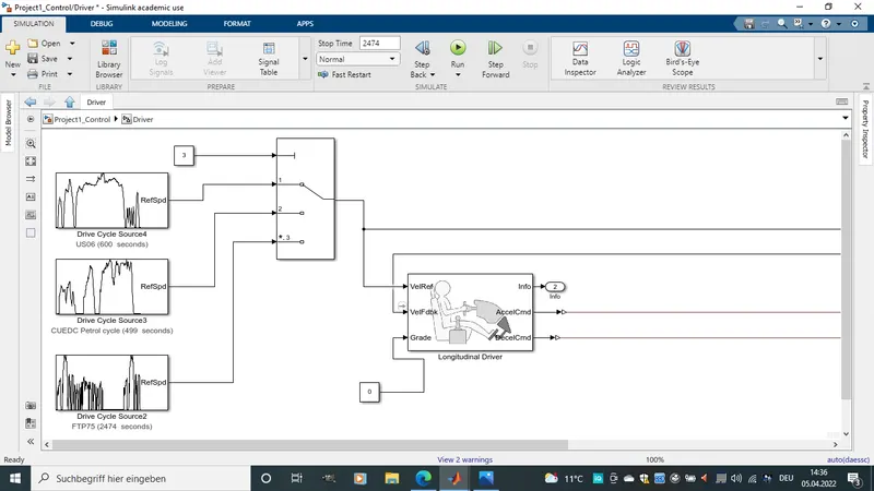
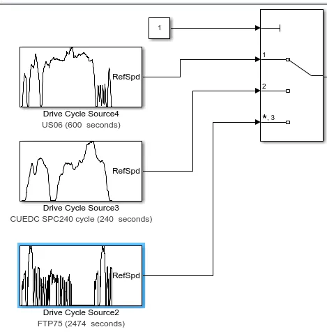
This subsytem contains Drive cycle inputs and a longitudinal driver. The drive cycle is just a predefine velocity in refference to time data. This data is then given to the longitudinal driver who the accelerates and deccelerate the vehicle in refference to input drive cycle.For this siulation three drive cycles are connected to a multi switch block, and a conctant block is given to choose which drive cycle the vehicle should follow.

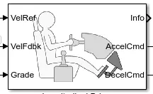
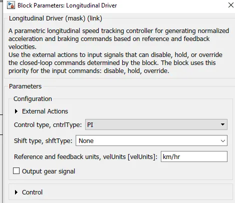
The Longitudinal Driver block implements a longitudinal speed-tracking controller. Based on reference and feedback velocities, the block generates normalized acceleration and braking commands that can vary from 0 through 1. You can use the block to model the dynamic response of a driver or to generate the commands necessary to track a longitudinal drive cycle.

Battery:

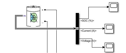
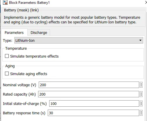
Here a battery is conected to supply the motor with power.Three scopes are connected to show battery state of charge, Current and voltage

EVALUATION:

Now one after the oder a simulation test will be carried on different drive cycles and observation on current,voltage,SOC and motor and controler tempirature will be made.

1) US06 (runing for 600sec)

Conclution:

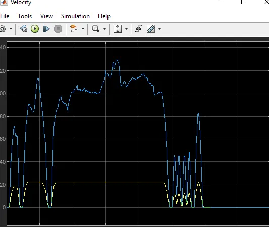
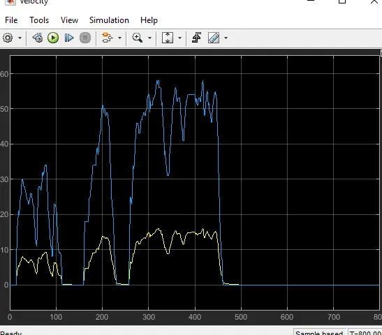
For this first cycle we could see from picture 1. The input velocity in blue and the vehicle velocity in yellow. The vehicle trying to follow the given input velocity. How ever it the dirrerence in both input and vehicle velocity is remarcable. This is due to the inability of the PI controler to to actualy correct the difference.

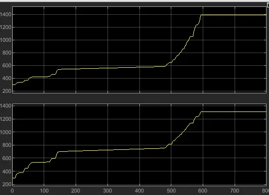
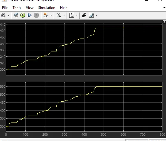
The second picture show motor and controler temperature change. we notice the sharp rice in temperature during acceleration. When the vehicle drives at constant speed the temperature is almost at constant.

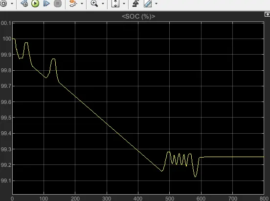
The third picture shows battery state. We see the battery charge during decceleration. When vehicle speeds up battery is consumed quicker but at constant speed there is a uniform battery consumtion.

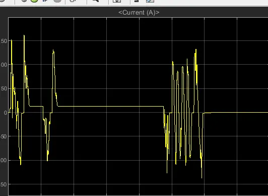
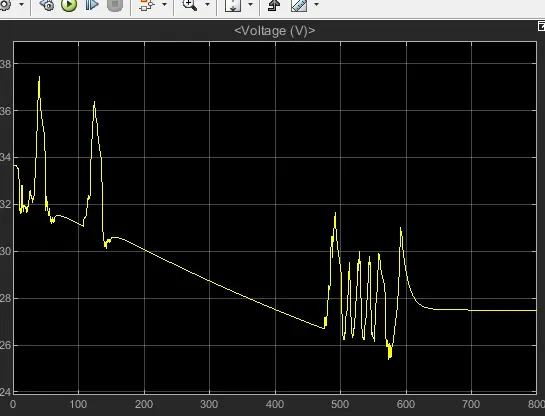
The tow last pictue for current and voltage respectively. Much more power is needed during acceleration reason why current and voltage go high in value during acceleration. At constant speed current is almost constant why voltage drops.

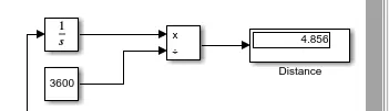
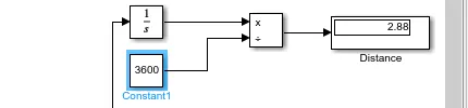
Below is a small model tu calculate distance covered fron the vehicle speed.

2) CUEDC Petrol cycle (499 sec)

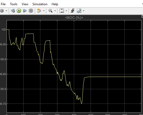
Conclution:

For this first cycle we could see from picture 1. The input velocity in blue and the vehicle velocity in yellow. The vehicle trying to follow the given input velocity. How ever it the dirrerence in both input and vehicle velocity is remarcable. This is due to the inability of the PI controler to to actualy correct the difference.

The second picture show motor and controler temperature change. we notice the sharp rice in temperature during acceleration. When the vehicle drives at constant speed the temperature is almost at constant.

The third picture shows battery state. We see the battery charge during decceleration. When vehicle speeds up battery is consumed quicker but at constant speed there is a uniform battery consumtion.

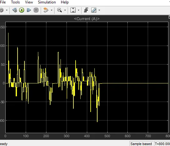
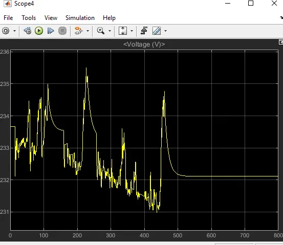
The tow last pictue for current and voltage respectively. Much more power is needed during acceleration reason why current and voltage go high in value during acceleration. At constant speed current is almost constant why voltage drops.

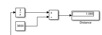
Below is a small model tu calculate distance covered fron the vehicle speed.

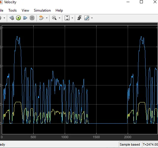
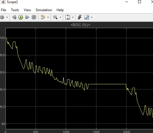
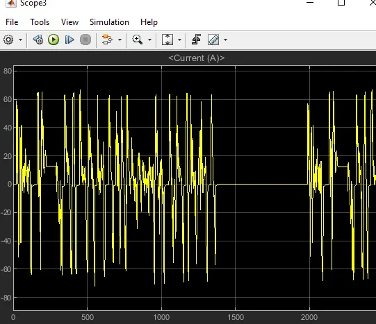
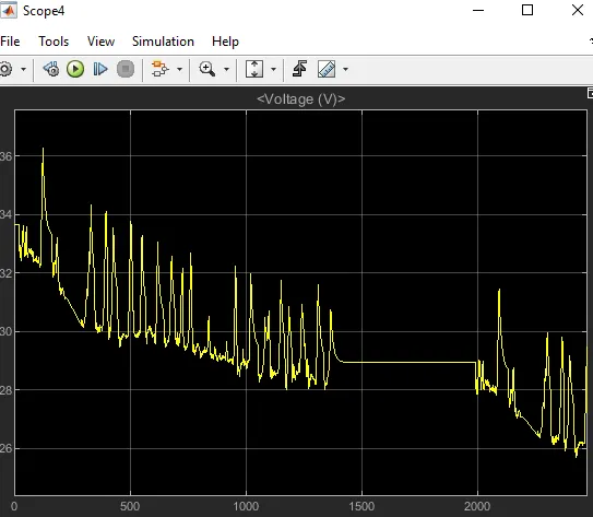
3) FTP75 (2474 sec)

Conclution:

For this first cycle we could see from picture 1. The input velocity in blue and the vehicle velocity in yellow. The vehicle trying to follow the given input velocity. How ever it the dirrerence in both input and vehicle velocity is remarcable. This is due to the inability of the PI controler to to actualy correct the difference.

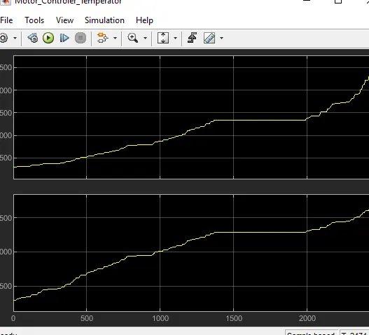
The second picture show motor and controler temperature change. we notice the sharp rice in temperature during acceleration. When the vehicle drives at constant speed the temperature is almost at constant.

The third picture shows battery state. We see the battery charge during decceleration. When vehicle speeds up battery is consumed quicker but at constant speed there is a uniform battery consumtion.

The tow last pictue for current and voltage respectively. Much more power is needed during acceleration reason why current and voltage go high in value during acceleration. At constant speed current is almost constant why voltage drops.

Below is a small model tu calculate distance covered fron the vehicle speed.