Final Project: Electric Rickshaw modelling

Final Project: Electric Rickshaw modelling

Create a detailed MATLAB model of an electric rickshaw (three wheel passenger vehicle) as per details below:

• Rear wheels driven by PM brushed type motor
• Assume efficiency points of motor controller and motor
• Make an excel sheet of all input and assumed data
• Results: For any three standard driving cycles show energy consumption, temperature rise of motor and controller for 100 km constant speed driving at 45 kmph.

(Note- The simulink model file should be compulsorily attached)

Speedy growth

E-rickshaws currently comprise 83 per cent of the India electric vehicle market.

India currently has around 15 lakh e-rickshaws that increase with additional sales of around 11,000 new ones every month. These figures could be much higher as a large percentage is still unregistered. The market is expected to witness a sale of 9.25 lakh e-rickshaw by 2024.

Environmental benefits: E-rickshaws help mitigate air and noise pollution. At least 1,036.6 tonnes of CO₂ emissions can be mitigated a day (378,357 tonne CO₂ annually) if compressed natural gas auto is replaced by e-rickshaws.

.

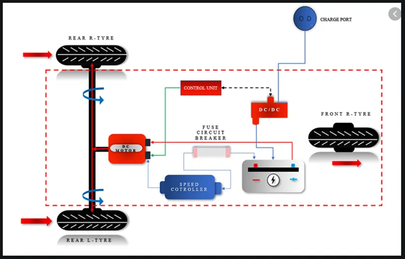
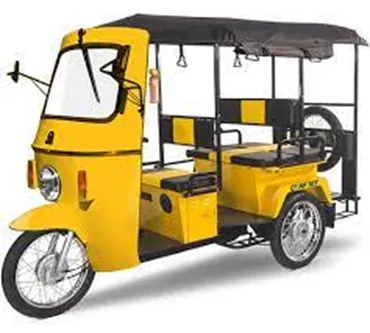
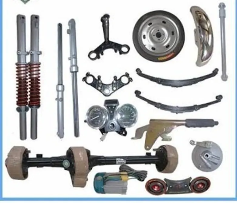
spare parts of E rickshaw

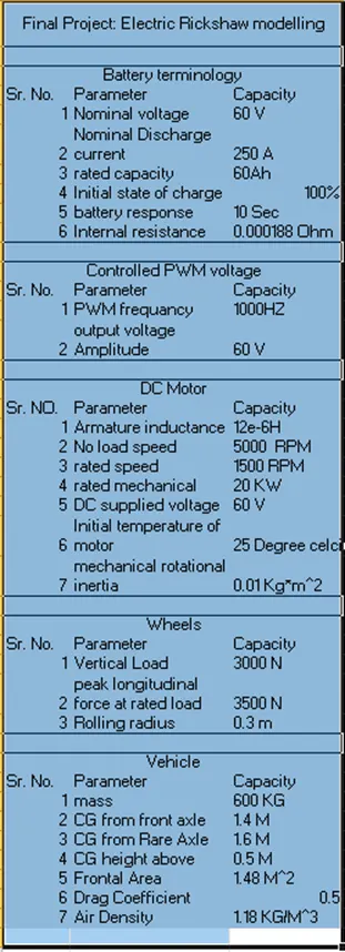
PROCUDURE:-

On above images we see outer look of electric Rickshaw as well as chassis components and spare parts required for Rickshaw

So we construct one by one component in metalab Simulink so

Step 1:- construction of Vehicle body and chassis

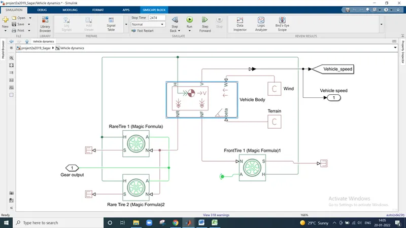
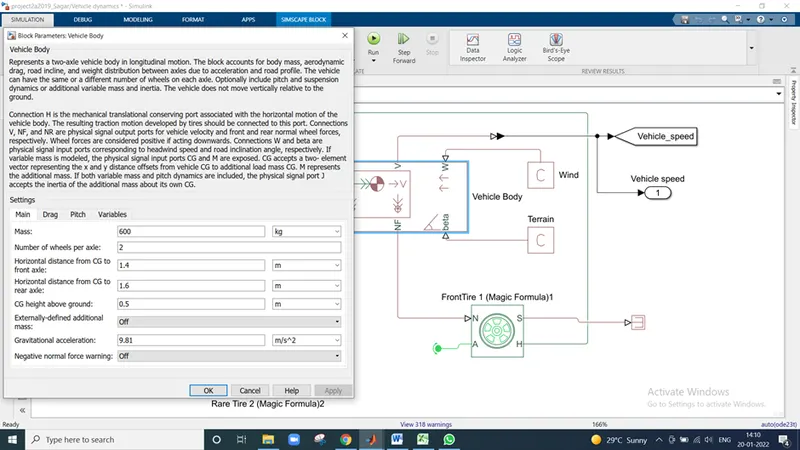
here we take vehicle body in simulation block with same assumption which is in present in axel file

Connection H is the mechanical translational conserving port associated with the horizontal motion of the vehicle body. The resulting traction motion developed by tires should be connected to this port. Connections V, NF, and NR are physical signal output ports for vehicle velocity and front and rear normal wheel forces, respectively. Wheel forces are considered positive if acting downwards. Connections W and beta are physical signal input ports corresponding to headwind speed and road inclination angle, respectively. If variable mass is modeled, the physical signal input ports CG and M are exposed. CG accepts a two- element vector representing the x and y distance offsets from vehicle CG to additional load mass CG. M represents the additional mass. If both variable mass and pitch dynamics are included, the physical signal port J accepts the inertia of the additional mass about its own CG.

WHEELS

Connection N is a physical signal input port that applies the normal force acting on the tire. The force is considered positive if it acts downwards. Connection S is a physical signal output port that reports the tire slip.

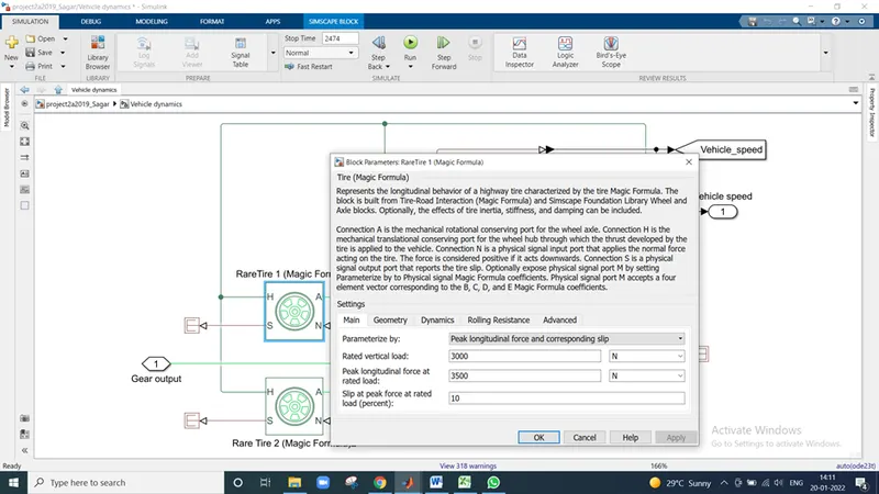
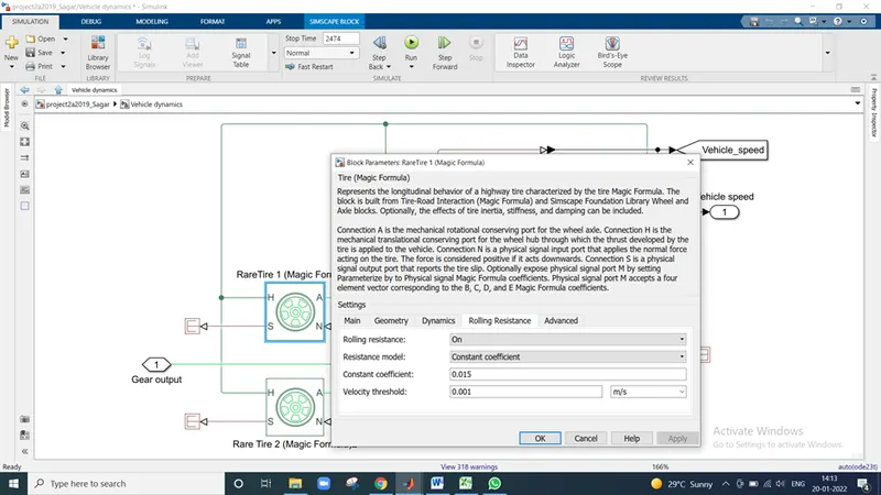
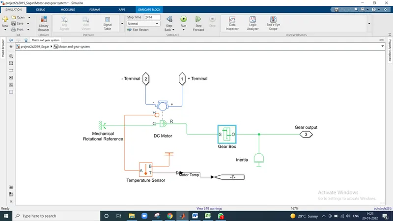
Here we seen the vehicle body no we construct the motor and gear system

STEP 2 :- CONSTRUCTION OF MOTOR AND GEAR SYSTEM

As per requirement we need PM brushed type motor

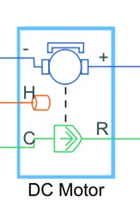
. Motor parameters can either be specified directly, or derived from no-load speed and stall torque.

When a positive current flows from the electrical + to - ports, a positive torque acts from the mechanical C to R ports. Motor torque direction can be changed by altering the sign of the back-emf or torque constants.

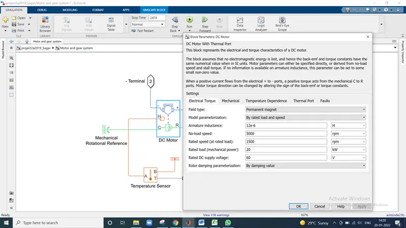
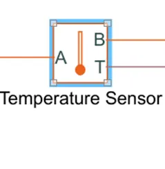
For controlling temperature of the motor we need temperature sensor

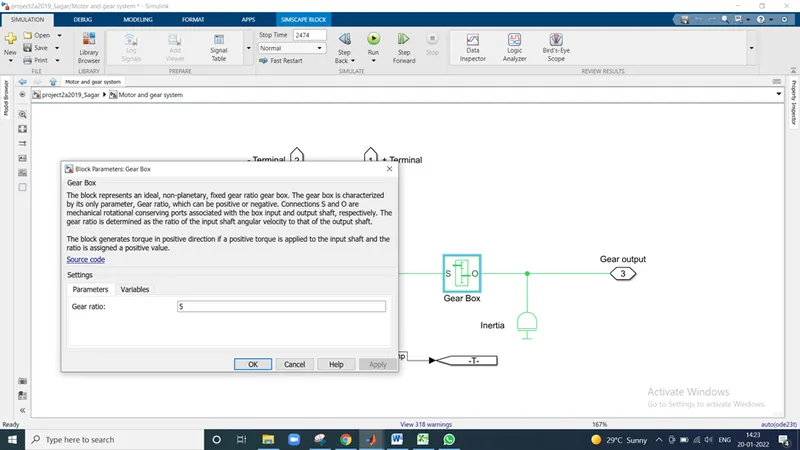
Gear Box

The block represents an ideal, non-planetary, fixed gear ratio gear box. The gear box is characterized by its only parameter, Gear ratio, which can be positive or negative. Connections S and O are mechanical rotational conserving ports associated with the box input and output shaft, respectively. The gear ratio is determined as the ratio of the input shaft angular velocity to that of the output shaft.

Now we required gear box for maintaining speed torque balance

Now we arrange all the date and connect

STEP 3 :- CONSTRUCTION OF POWER CONYTROLLER

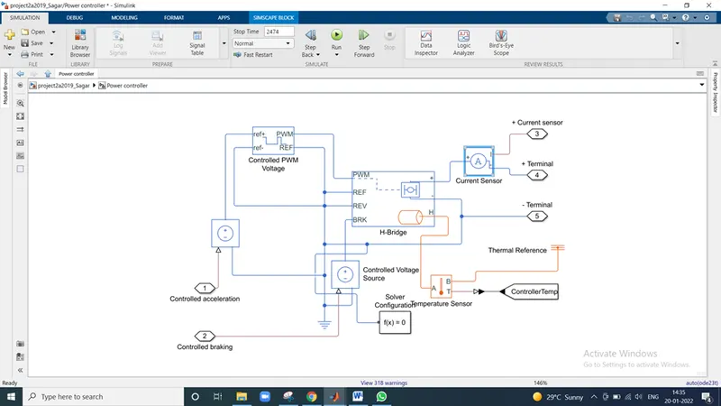
Here we required

1. Controlled PWM voltage
2. H- Bridge
3. Temperature sensor
4. Current sensor
5. Thermal reference
6. Controlled source

• Controlled PWM voltage

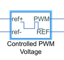
This block creates a Pulse-Width Modulated (PWM) voltage across the PWM and REF ports. The output voltage is zero when the pulse is low, and is equal to the Output voltage amplitude parameter when high.

• H- Bridge

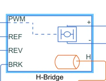
This block represents an H-bridge motor drive. The block can be driven by the Controlled PWM Voltage block in PWM or Averaged mode. In PWM mode, the motor is powered if the PWM port voltage is above the Enable threshold voltage. In Averaged mode, the PWM port voltage divided by the PWM signal amplitude parameter defines the ratio of the on-time to the PWM period. Using this ratio and assumptions about the load, the block applies an average voltage to the load that achieves the correct average load current

If the REV port voltage is greater than the Reverse threshold voltage, then the output voltage polarity is reversed.

If the BRK port voltage is greater than the Braking threshold voltage, then the output terminals are short circuited via one bridge arm in series with the parallel combination of a second bridge arm and a freewheeling diode

Now we check the design of power controller

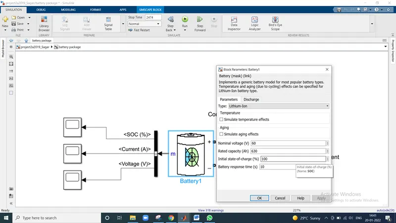
STEP 4 :- DESIGN OF BATTERY

Here we use

1. Generic battery model
2. Power gui
3. Controlled current source
4. Bus selector
5. scopes

STEP 5 :- DESIGN OF DRIVER PARAMETAR

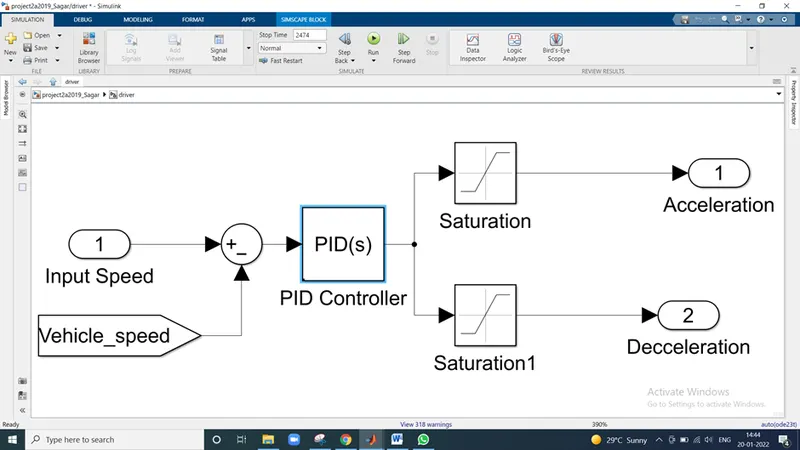
Here we use PID controller and saturation curve

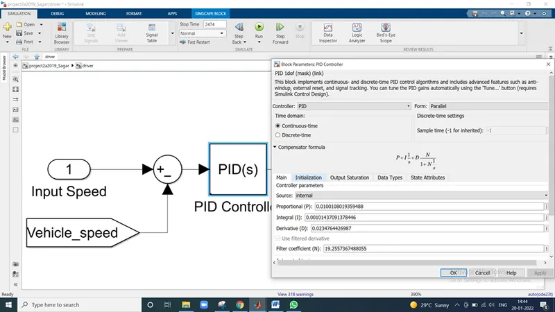
Which is guide acceleration and deceleration

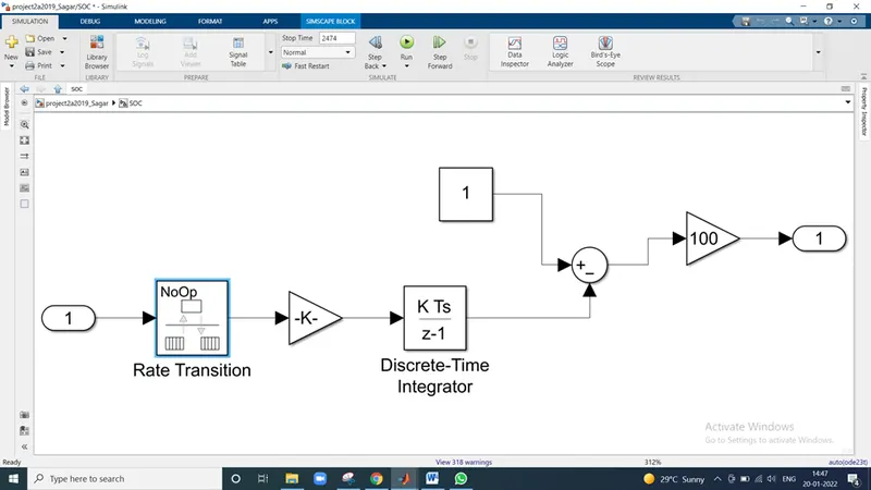
Now we check the vehicle model connections

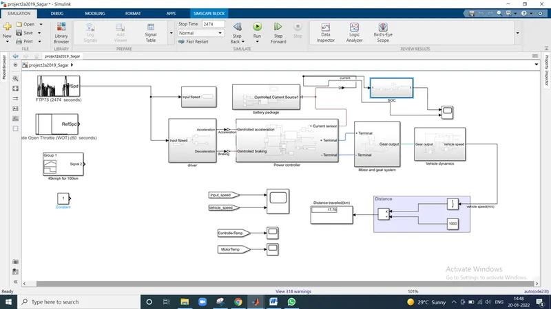
Here we see the connection of E rickshaw now goes to scope result

Result :-

• For FTP 75 in 2474 ses Rickshaw travel 17.38 Km distance
• 

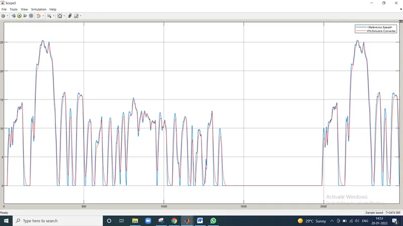
Here reference speed and PS- simulation speed is nearly same at starting condition vehicle need more power so graph show high deflection

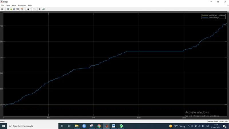
Here we seen that motor temperature is increases gradually but PS temperature is not me shows deflection so we check in single scope

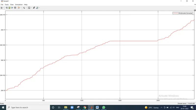
Here we see the temperature is 298.15 to 298.173 of PS simulation motor

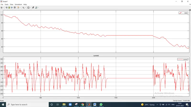
• For wide open Throttle for 60 sec rickshaw travel 0.47 Km

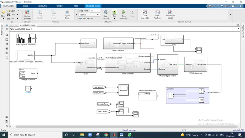
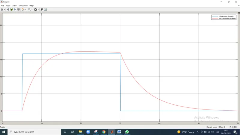
here we see the PS simulation speed is greater than reference because at stating condition vehicle required more power then its run on normal speed

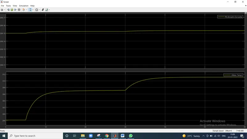
Here again motor temperature shows more deflection than simulation

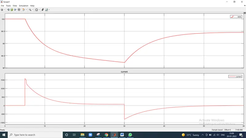
Here after 4 sec vehicle will start in running so soc reduce and current linearly increase in vertical because of acceleration but after 10 sec its will increases linearly

• For signal Builder

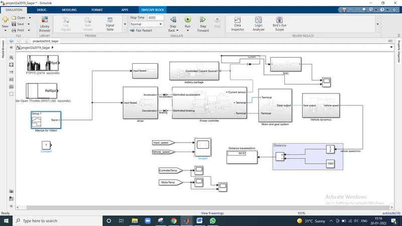
For 45 kmph speed Rickshaw travel 99.97 Km in 8000 sec

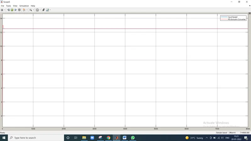
Due to constant speed journy the graph speed is linear to reference speed

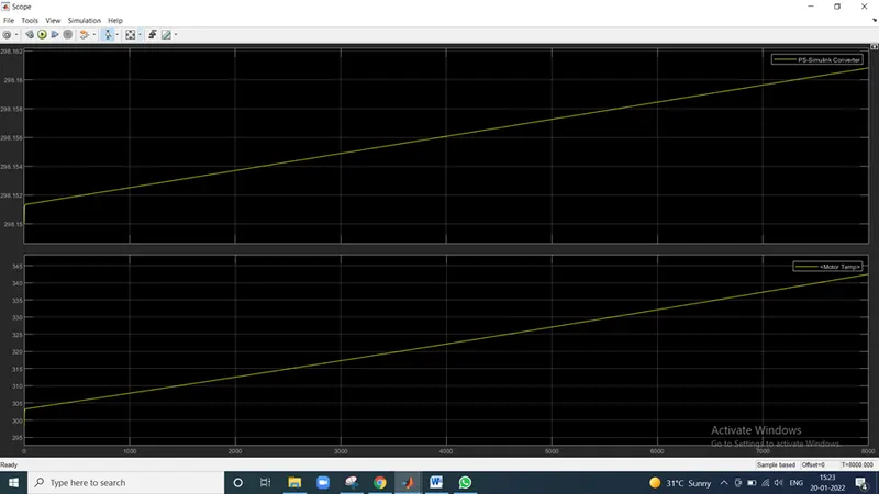
Constant speed and no acceleration or deceleration motor temperature and reference temperature are gradually increases motor temperature 342 k

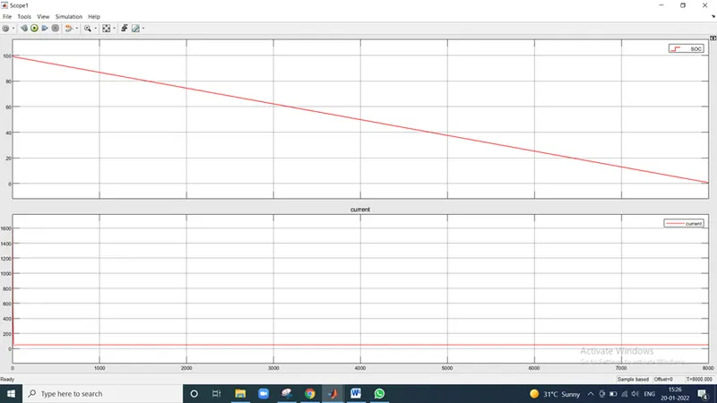
Constant speed journey so battery completely drain and current are constant

Conclusion :- Hence Design of E- Rickshaw Completed Succesfully