Design of an Electric Vehicle.
Aim: Create a MATLAB model of an electric car that uses a battery and a DC motor.
Objective:
-
System-level configurations
-
Model parameters
-
Reviewing results or outputs
Introduction of Electric Car:
An electric car is a car that is propelled by one or more electric motors, using energy stored in rechargeable batteries. Compared to internal combustion engine (ICE) vehicles, electric cars are quieter, have no exhaust emissions, and lower emissions overall. In the United States, as of 2020, the total cost of ownership of recent EVs is cheaper than that of equivalent ICE cars, due to lower fueling and maintenance costs. Charging an electric car can be done at a variety of charging stations; these charging stations can be installed in both houses and public areas.
Several countries have established government incentives for plug-in electric vehicles, tax credits, subsidies, and other non-monetary incentives. Several countries have established a phase-out of fossil fuel vehicles, and California, which is one of the largest vehicle markets, has an executive order to ban sales of new gasoline-powered vehicles by 2035. The Tesla Model 3, which has a maximum range of 570 km (353 miles) according to the EPA, has been the world's best-selling electric vehicle (EV) on an annual basis since 2018 and became the world's all-time best-selling electric car in early 2020.
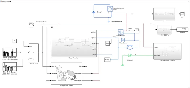
Matlab model of an electric car:
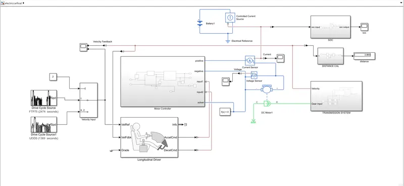
Blocks used in this model:
- Tire(magic formula)
- Vehicle body
- Dc motor
- H-Bridge converter
- Controlled PMW voltage
- Longitudinal driver
- Battery
- Controlled current source
- Current, Voltage sensors
- Multi-port switch
- Drive cycle( FTP75, UDDS)
Blocks explanation:
1.Tire(magic formula)
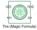
The Tire (Magic Formula) block models a tire with longitudinal behaviour given by the Magic Formula, an empirical equation based on four fitting coefficients. The block can model tire dynamics under constant or variable pavement conditions. The longitudinal direction of the tire is the same as its direction of motion as it rolls on the pavement. This block is a structural component based on the Tire-Road Interaction (Magic Formula) block. To increase the fidelity of the tire model, you can specify properties such as tire compliance, inertia, and rolling resistance. However, these properties increase the complexity of the tire model and can slow down the simulation. Consider ignoring tire compliance and inertia if simulating the model in real-time or if preparing the model for hardware-in-the-loop (HIL) simulation.
Ports: N - Normal force on the wheels.
S - Slip angle between tire and road
H - Wheel hub
A - Axle on which tires sits on
2.Vehicle body
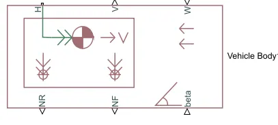
The Vehicle Body block represents a two-axle vehicle body in longitudinal motion. The vehicle can have the same or a different number of wheels on each axle. For example, two wheels on the front axle and one wheel on the rear axle. The vehicle wheels are assumed identical in size. The vehicle can also have a centre of gravity (CG) that is at or below the plane of travel. The block accounts for body mass, aerodynamic drag, road incline, and weight distribution between axles due to acceleration and road profile. Optionally include pitch and suspension dynamics. The vehicle does not move vertically relative to the ground. The block has an option to include an externally defined mass and an externally defined inertia. The mass, inertia, and centre of gravity of the vehicle body can vary over the course of simulation in response to system changes.
Input ports:
- W - Headwind speed (m/s)
- beta - Road incline angle(rad)
- CG - Centre of gravity(m)
- M - Mass(kg)
- J - External moment of inertia(kg*m^2)
Output ports:
- V - Longitudinal velocity(m/s)
- NF - Front axle normal force(N)
- NR - Rear axle normal force(N)
Conserving port:
- H - Horizontal motion
3.DC motor
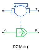
The DC Motor block represents the electrical and torque characteristics of a DC motor using the following equivalent circuit model:
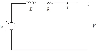
The resistor R corresponds to the resistance you specify in the Armature resistance parameter. The inductor L corresponds to the inductance you specify in the Armature inductance parameter. DC motor block is used to supply propulsion power to the wheel through the gearbox. There are various types of DC motor block such as BLDC, PMDC, etc based on the propulsion requirement proper motor is used as per the voltage supply conditions.
Electrical ports:
- -: Negative terminal
- +: Positive terminal
Mechanical ports:
- R - Motor rotor
- C - Motor case
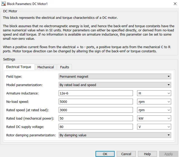
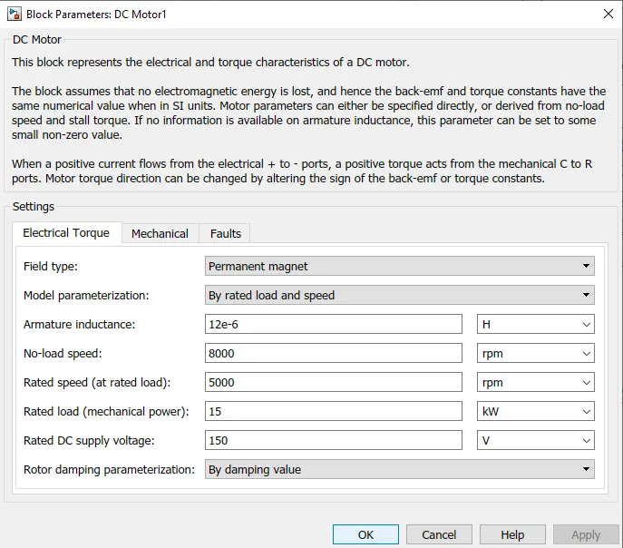
As DC motor block contains two parts one is electrical and another is mechanical. The electrical part is connected to the controller port and the machine is connected to the gearbox and electrical reference. The parameters of the DC motor can be changed as per the required conditions. Here we have chosen as rated power and no-load speed. As the rated power in an electric vehicle is in kW so we change W to kW and it is a range of 50-100 we have kept here as 50kW of rated power. According to vehicle speed and gear ratio rated speed can be changed here we have taken as 3000rpm as the rated speed of the motor and no-load speed as 5000 rpm. The battery pack contains various cells of 3.6kW of power each and are connected in series and parallel combination for supplying the power supply voltage as per the rated power. Here we have taken the rated DC supply voltage as 80 V.
4.H-Bridge converter
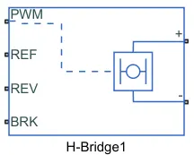
The H-Bridge block represents an H-bridge motor driver. The block has the following two Simulation mode options:
-
PWM — The H-Bridge block output is a controlled voltage that depends on the input signal at the PWM port. If the input signal has a value greater than the Enable threshold voltage parameter value, the H-Bridge block output is on and has a value equal to the value of the Output voltage amplitude parameter. If it has a value less than the Enable threshold voltage parameter value, the block maintains the load circuit using one of the following three Freewheeling mode options:
-
Via one semiconductor switch and one freewheeling diode.
-
Via two freewheeling diode
-
Via two semiconductor switches and one freewheeling diode
The first and third options are sometimes referred to as a synchronous operation.
The signal at the REV port determines the polarity of the output. If the value of the signal at the REV port is less than the value of the Reverse threshold voltage parameter, the output has positive polarity; otherwise, it has negative polarity.
-
-
Averaged— This mode has two Load current characteristics options:
-
Smoothed
-
Unsmoothed or discontinuous
The smoothed option assumes that the current is practically continuous due to load inductance. In this case, the H-Bridge block output is:
`(V_oV_(PWM))/A_(PWM)-I_(out)R_(on)`
where:
-
`V_o` is the value of the Output voltage amplitude parameter.
-
`V_(PWM)` is the value of the voltage at the PWM port.
-
`A_(PWM)` is the value of the PWM signal amplitude parameter.
-
`I_(out)` is the value of the output current.
-
`R_(on)` is the Bridge on the resistance parameter.
-
Ports:
- -: Negative load connection port
- +:Positive load connection port
- V-:Negative voltage connection
- V+:Positive voltage connection
- PWM: pulse width modulated signal
- ref: Reference
- REV: Reverse
- BRK: Brake
- H: Thermal
5.Controlled PMW voltage
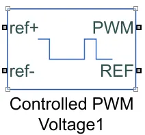
The Controlled PWM Voltage block represents a pulse-width modulated (PWM) voltage source. The block has two modelling variants, accessible by right-clicking the block in your block diagram and then selecting the appropriate option from the context menu, under Simscape >Block choices:
-
Electrical input ports — The block calculates the duty cycle based on the reference voltage across its ref+ and ref- ports. This modelling variant is the default.
-
PS input — Specify the duty cycle value directly by using an input physical signal port.
For the Electrical input ports variant of the block, the demanded duty cycle is
`100∗(V_(ref)−V_(min))/(V_(max)−V_(min))`
where:
-
Vref is the reference voltage across the ref+ and ref- ports.
-
Vmin is the minimum reference voltage.
-
Vmax is the maximum reference voltage.
Ports:
- ref+: Positive terminal
- ref-: Negative terminal
- REF - Floating zero volt reference
- PWM - Pulse width modulated signal
6.Longitudinal driver
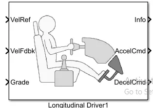
The Longitudinal Driver block implements a longitudinal speed-tracking controller. Based on reference and feedback velocities, the block generates normalized acceleration and braking commands that can vary from 0 through 1. You can use the block to model the dynamic response of a driver or to generate the commands necessary to track a longitudinal drive cycle.
Input ports:
- VelRef: Reference vehicle velocity
- VelFdbk: Longitudinal vehicle velocity
- Grade: Road grade angle
- EnblAccelOvr: Enable acceleration command override
- AccelOvrcmd: Acceleration override command
- AccelHld: Acceleration Hold command
- AccelZero: Disable acceleration command
- EnblDecelOvr: Enable deceleration override command
- DecelOvrCmd: Deceleration override command
- DecelHld: Deceleration Hold command
- Decelzero: Disable deceleration command
- Extgear: Gear
output ports:
- Info: Bus signal
- AccelCmd: Commanded vehicle acceleration
- DecelCmd: Commanded vehicle deceleration
- Gearcmd: Commanded vehicle gear
7.Controlled current source
The Controlled Current Source block represents an ideal current source that is powerful enough to maintain the specified current through it regardless of the voltage across the source. The output current is I = Is, where Is is the numerical value presented at the physical signal port. The positive direction of the current flow is indicated by the arrow.
Vehicle model Subsystems:
1.Transmission system
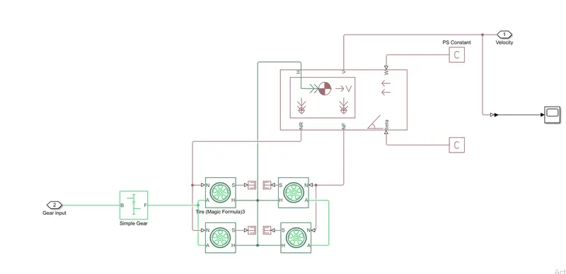
Explanation:
- As we know transmission is the main part of the vehicle which is used to supply the propulsion powers from the motor and the battery to the wheels.
- Under transmission, the part number of components come which are wheels, gearbox, throttle, power input etc.
- In this transmission subsystem blocks used are Tire, vehicle body, simple gearbox block.
- There are 4 tire blocks used as 4 wheels of the vehicle and here we have connected the gearbox with the rear wheel to make it a rear-wheel drive.
- The vehicle body block is been connected to these wheels by all the input and output ports.
- In-vehicle body block we have connected as ps constant block to beta and wind velocity as we have assumed both as zero and hub motor port is also connected with the wheels H port.
2.Motor controller
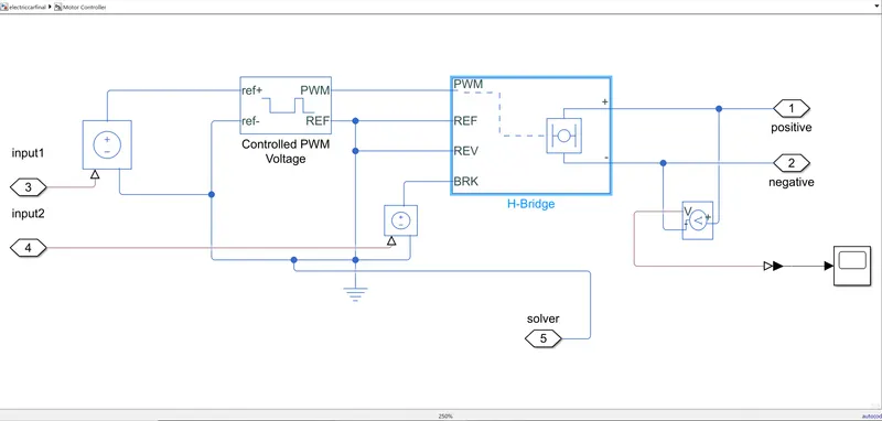
Explanation:
- This motor controller subsystem contains H-Bridge and a Controlled PWM Voltage block.
- H-Bridge block is used to supply the power from the battery to the DC motor.
- H-Bridge has 4 switches that give the controlled DC voltage supply to the DC motor and we can also control the supply of voltages.
- In H-Bridge we have control on PWM voltage, Reverse and braking effect also.
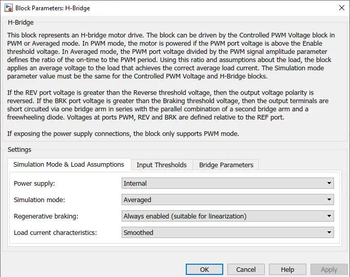
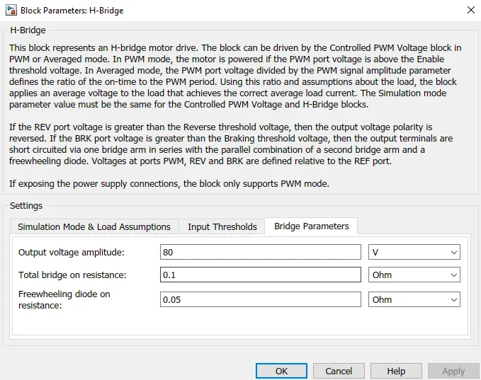
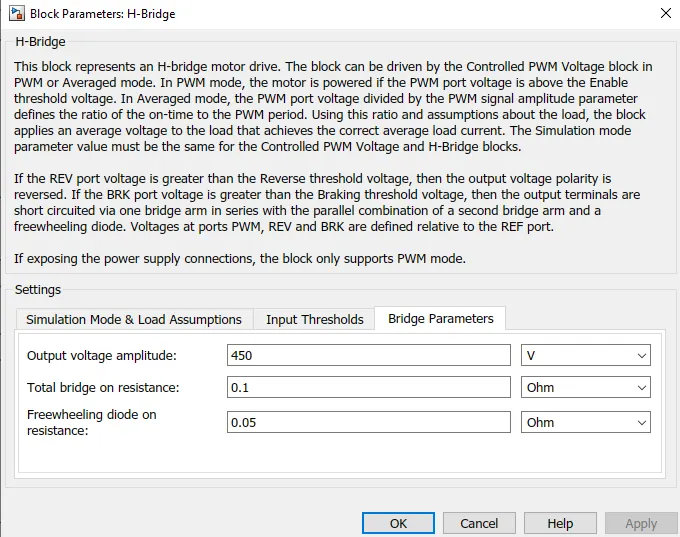
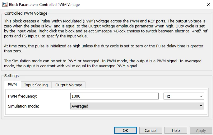
- As below we can see block parameters, for simulation mode we have two options internal and external as we choose internal we have a choice of PWM mode and averaged mode.
- In PWM mode the simulation time increases drastically as if the simulation time is of 5 secs then PWM mode is effective but as now our simulation time is in mins or hours so here averaged mode is been chosen as it is faster compared to PWM mode.
- Also, we have kept regenerative mode enable and load current characteristics as smoothed.
- Also, we have to change the output voltage amplitude to the voltage we have supplied to the DC motor.
- As from the Controlled PWM voltage block which is connected to the input PWM Pin in the H-Bridge block.
- This block will apply pulses and based on these pulses from the fixed battery voltage variable output voltage will be available to the motor and the motor speed and motor torque are changed.
- So basically this subsystem will control the power supply to the DC motor using the following blocks.
3.SOC calculation
Explanation:
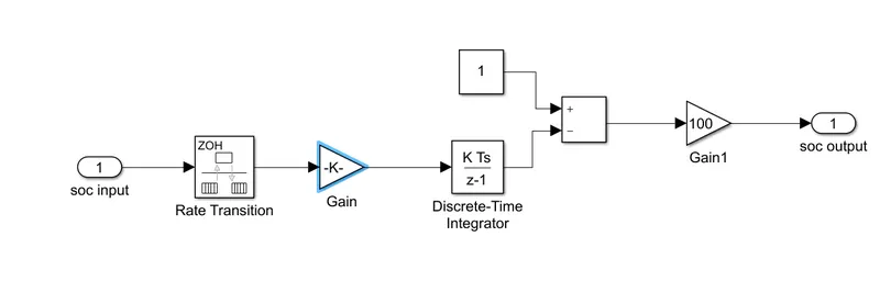
- Here in this subsystem, there is the number of blocks used are rate transition, gain, constant, add, etc.
- Rate transition block takes input from the controlled current source block as soc input signals and do a sampling of the signals and gives to gain block.
- Gain block multiplies the sampling signal with the rated voltage and gives it to the discrete-time integrator block.
- Discrete-time integrator block integrates the signal and adds it to the constant given and supply is to the gain block again.
- Gain block multiplies it with the 100 and gives it to the SOC output.
4.Distance calculation
Explanation:
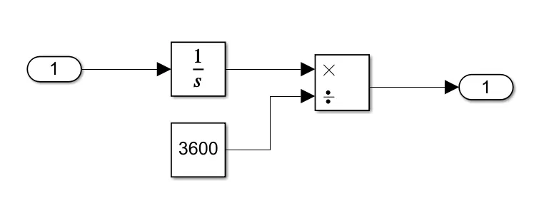
- Here the input is taken from the velocity feedback and it is integrated using the integrator block and divided with 3600 to get output per seconds.
1.FTP75 Drive cycle as input:
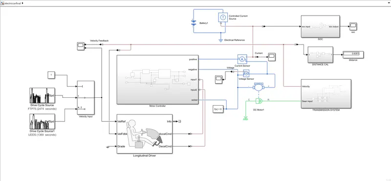
Input parameter:
Output: SOC plot
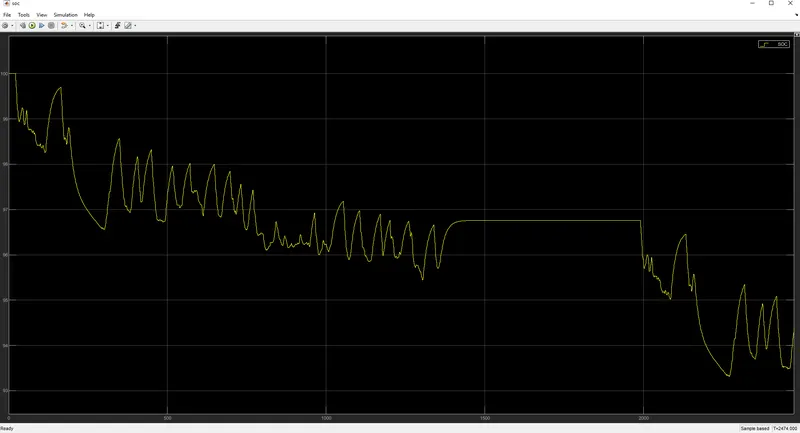
Result:
- Here we gave the input as FTP75 drive cycle and run the model for 2474 sec.
- So here we can observe the SOC of the battery is been discharged by 17% of the total 100% battery charge.
- SOC of the battery is 83% after the drive cycle is completed.
- AS we observe the graph at the graph is not at a steady-state sometimes it is going up and sometimes it's going down, while the curve is going down means the battery is getting discharged and while the curve is going up it means the battery is getting charged again.
- The battery is getting charged due to regenerative braking.
- From 1200sec to 2000 sec the battery is changing continuously.
Output: Distance travelled
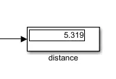
Result:
- Distance travelled by the vehicle is 5.319km for the applied voltage of 80V.
- This distance is calculated using velocity feedback given.
Output: Velocity
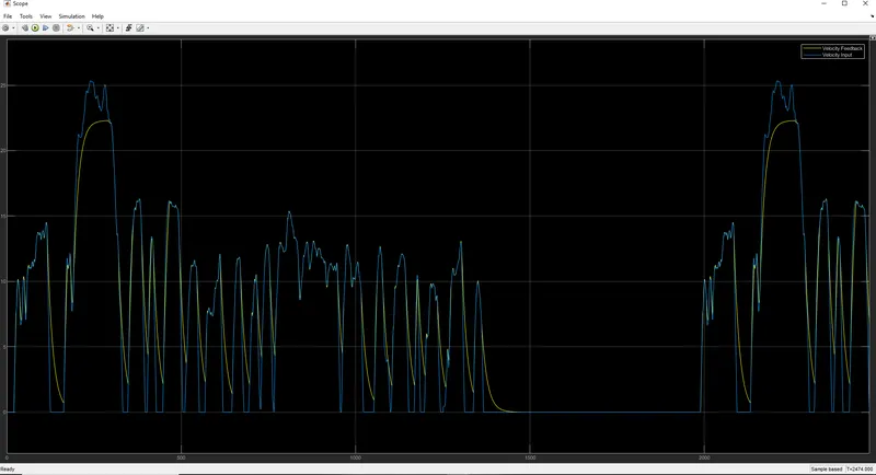
Result:
- As the input given to the vehicle velocity was the FTP75 drive cycle.
- Here we can observe that velocity by the vehicle is approximately the same as of standard drive cycle given as input.
- As here we can observe while steep braking of the vehicle, our vehicle takes more time for the braking as the standard drive cycle.
- While acceleration also vehicle takes comparatively more time to get at that peak velocity.
- As per the standard drive cycle peak velocity attained by the vehicle is 25m/s but the velocity traced by the vehicle is about 22m/s which is 30% less than standard drive cycle velocity.
2. UDDS cycle as input:
Input parameters:
Output: SOC plot
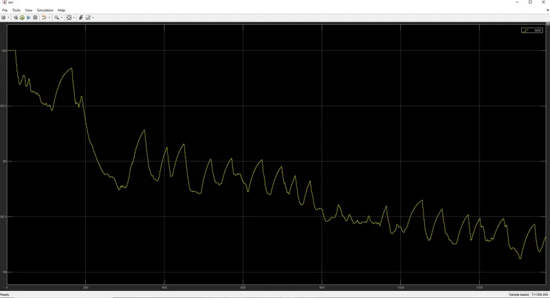
Result:
- Here we gave the input as UDDS drive cycle and run the model for 1369 sec.
- So here we can observe the SOC of the battery is been discharged by 8% of the total 100% battery charge.
- SOC of the battery is 92% left after the drive cycle is completed.
- AS we observe the graph at the graph is not at a steady-state sometimes it is going up and sometimes it's going down, while the curve is going down means the battery is getting discharged and while the curve is going up it means the battery is getting charged again.
- The battery is getting charged due to regenerative braking.
Output: Distance travelled
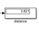
Result:
- Distance travelled by the vehicle is 3.821 km for the applied voltage of 150V DC motor voltage and H-Bridge voltage is 450V.
- This distance is calculated using velocity feedback given.
Output: Velocity plot
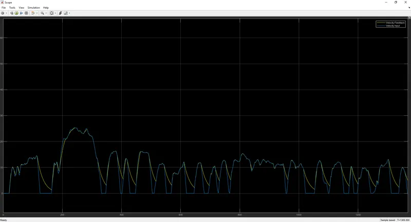
Result:
- As the input given to the vehicle velocity was the UDDS drive cycle.
- Here we can observe that velocity by the vehicle is approximately the same as of standard drive cycle given as input.
- As here we can observe while steep braking of the vehicle, our vehicle takes more time for the braking as the standard drive cycle.
- In this, the PWM frequency is being increased to 1000 Hz for the desired output.
- In this plot as we can observe the braking of the vehicle is not being so much satisfied as that of velocity increase.
---------------------------------------------------------------------------------------------------------------------------------------------------------------
Conclusion:
| Input | Distance covered(km) | Peak Velocity(m/s) | SOC(%) |
| 1.FTP75 | 5.319 | 22 | 83 |
| 2.UDDS | 3.812 | 25 | 92 |