Final Project: Design of an Electric Vehicle
PROJECT - 2
DESIGN OF AN ELECTRIC VEHICLE
Theory:
An electric vehicle (EV) is characterized by its use of an electric motor or traction motor for propulsion, diverging from the internal combustion engines typical in conventional vehicles. EVs rely on electricity rather than fossil fuels, leading to reduced emissions and pollution. Power for EVs is sourced from batteries, generators, or other collector systems, with batteries featuring high energy densities to meet power demands and extend range.
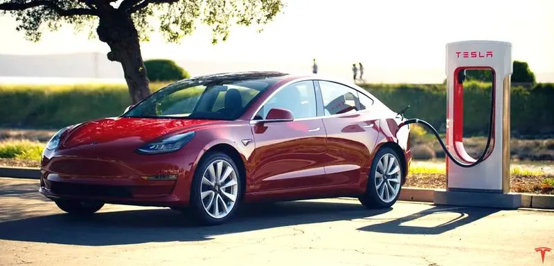
The power output of an EV's electric motor, measured in kilowatts (kW), is comparable to conventional vehicles, typically rated in horsepower (hp). While 100 kW equates to roughly 134 hp, electric motors exhibit superior torque delivery across a wide RPM range compared to internal combustion engines, which are limited in their torque output within specific engine speeds. However, energy conversion from electrical to mechanical energy results in some losses, with around 90% efficiency observed in the conversion process, with losses occurring mainly in the motor and drivetrain components.
The electrification process commonly involves converting direct current (DC) electricity into alternating current (AC) using a DC/AC inverter, which is then supplied to a 3-phase AC motor. While electric trains and certain electric vehicles utilize DC motors, others may employ universal motors capable of operating with both AC and DC power sources. Various motor types, including induction motors and permanent magnet machines, are integrated into modern production vehicles, such as Tesla Motors' use of induction motors and the utilization of permanent magnet machines in vehicles like the Nissan Leaf and Chevrolet Bolt.
Many electric transport systems draw power from stationary electricity sources connected directly to vehicles via wires. This setup enables regenerative braking, where motors function as brakes and generators, converting kinetic energy into electrical power, which can be fed back into the system. Regenerative braking proves particularly beneficial in mountainous terrains, as descending vehicles can contribute to power generation required for ascending vehicles. However, for EVs to gain widespread adoption, convenient charging infrastructure is essential, necessitating the establishment of numerous charging stations, ideally supplemented by solar-powered residential setups. EVs typically command higher costs due to expensive battery and electric component technologies.
Hybrid electric vehicles (HEVs) combine internal combustion engines with electric propulsion systems, aiming to enhance fuel economy and overall performance. HEVs utilize electric power to supplement conventional fuels, either by charging batteries or powering electric drive motors directly through motor-generator units. Additionally, HEVs incorporate regenerative braking to replenish battery charge. While EVs represent a smaller share of the global automotive market, around 2-3%, HEVs command a larger market share, accounting for approximately 19% of all automobiles sold worldwide. The Toyota Prius stands out as the best-selling HEV to date.
In the subsequent sections of this report, I will develop a simulation model of an electric vehicle equipped with a DC motor and battery system using SIMULINK software. The model will simulate a drive cycle, capturing velocity profiles, current dynamics, and battery state of charge characteristics. Various components necessary for the simulation will be represented as blocks within the SIMULINK block library.
AIM
The aim of this project is to create a MATLAB model of an electric car utilizing a battery and a DC motor using the Powertrain Blockset.
OBJECTIVE
The objective is to develop a MATLAB model of an electric car employing the Powertrain Blockset, and subsequently, prepare a comprehensive report encompassing the following aspects:
1. System-level configurations
2. Model parameters
3. Results
4. Conclusion
DESIGN CALCULATIONS
To construct the electric vehicle (EV) model, several parameters such as power, energy, range, motor rating, battery capacity, etc., need to be calculated. We will refer to the specifications of the TATA NEXON EV for vehicle dimension data, as outlined below:
TATA NEXON EV – Specifications
- Power: 95 kW
- Length (mm): 3993
- Width (mm): 1811
- Height (mm): 1606
- Tire Dimension: 664.4 mm
- Kerb Weight (Kg): 1400
- Battery Capacity: 30.2 kWh
- Motor Ratings (3-phase PMSM): 97.46 kW, 245 Nm
- Range: 312 km
To determine the motor ratings, battery capacity, maximum power, torque, and energy required by the vehicle, a model must be created initially for the electric vehicle design.
Drive Cycle
The Worldwide harmonized Light vehicles Test Procedure (WLTP) is a standardized test procedure used to measure pollutants, CO2 emissions, and fuel consumption of traditional, hybrid, and electric vehicles. The WLTP procedure incorporates various driving cycles, including:
1. Class 1: Low power vehicles with PWr <= 22
2. Class 2: Vehicles with 22 < PWr <= 34
3. Class 3: High-power vehicles with PWr > 34
Where PWr [kW/Tonne] denotes the power-to-weight ratio, calculated as the ratio between the rated engine power and kerb weight.
Since we are modeling the TATA Nexon EV, parameters from the provided specifications will be used. With Pmax = 95 kW and Kerb Weight = 1.4 Tonnes, the power-to-weight ratio (PWr) is calculated as:
PWr = Pmax / mv = 95 / 1.4 = 67.85
As the vehicle's PWr exceeds 34, the WLTC Class 3 driving cycle will be utilized to compute energy consumption.
WLTC Class 3
The WLTC Class 3 consists of four sub-parts, each with a different maximum speed:
1. Low: up to 56.5 km/h
2. Medium: up to 76.6 km/h
3. High: up to 97.4 km/h
4. Extra-high: up to 131.3 km/h
These driving phases simulate urban, suburban, rural, and highway scenarios, with an equal division between urban and non-urban paths (52% and 48%).
Force Calculation
The forces acting on the vehicle include:
1. Rolling Resistance
2. Aerodynamic Drag
3. Grade Resistance
4. Acceleration Resistance
The total force is the sum of all the above forces, and power, torque, and energy can be calculated accordingly.
The Vehicle Model in Simulink will be translated into a Simulink model, as illustrated below.
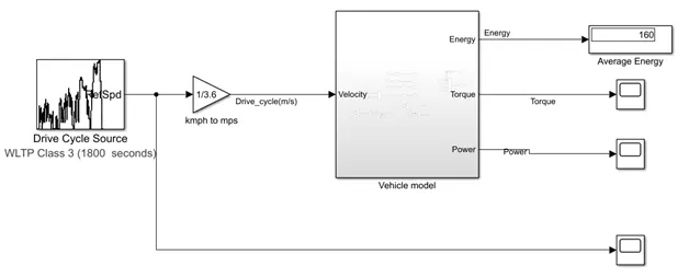
By dividing the last calculated value of the total energy by the total length of the WLTC drive cycle (23.266 km), we can obtain the average energy consumption of the vehicle, which is 160 Wh/km.
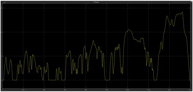
The power curve of the vehicle, as depicted Above, illustrates the power required at different speeds during the drive cycle. From this plot, it is evident that to attain the maximum speed of 131 km/hr, the motor should ideally be rated at 140 kW. However, due to size and cost constraints, selecting a high-rated motor may not be feasible. Therefore, the motor should be chosen to operate at maximum efficiency during average speeds.
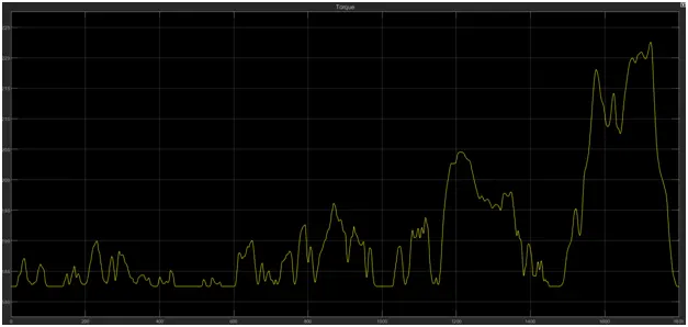
The torque curve, shown below, indicates that the maximum required torque is 222 Nm.
Motor Capacity Selection
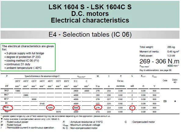
Based on the torque and power plots, a suitable motor for the Electric Car can be selected. Since we are modeling the TATA Nexon, a BLDC motor with the following specifications can be chosen:
- Rated Power: 95.8 kW
- Rated Torque: 279 Nm
- Rated voltage: 460V
- No load Speed: 3280 rpm
- Rated Speed: 4000 rpm
- Armature Inductance: 2mH
Battery Capacity Calculations
The average energy consumption for propulsion (Ep) is calculated as 160 Wh/km on the WLTC drive cycle. In addition to the energy needed for propulsion, the high voltage battery must supply energy for the vehicle’s auxiliary devices (Eaux) such as the 12V electrical system, heating, and cooling. We also need to consider the efficiency of the powertrain (ηp) during the conversion from electrical energy to mechanical energy.
The average electrical loads, including headlights and multimedia, consume approximately 430 W of electrical power. Over the duration of the WLTC cycle (1800 s or 0.5 h), this results in an energy consumption of 215 Wh for auxiliary loads. Dividing this by the length of the WLTC driving cycle (23.266 km) yields an average energy consumption for auxiliary loads (Eaux) of 9.241 Wh/km.
The overall average energy consumption (Eavg) is calculated using Equation (1), taking into account both propulsion and auxiliary loads. Considering an efficiency (ηp) of 0.9, we arrive at an average energy consumption of 188.045 Wh/km.
The battery pack is designed for a vehicle range of 250 km, resulting in a total energy requirement (Ebp) of 47.011 kWh. Following this, the number of battery cells connected in series (Ncs) is calculated, and subsequently, the energy content of a string (Ebs) and the total number of strings (Nsb) are determined.
SIMULINK MODELLING OF COMPLETE ELECTRIC VEHICLE
Main Simulation Diagram:
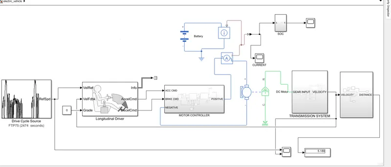
The Complete model of Electric vehicle in Simulink is as shown below.
COMPONENTS:
The main components of the EV are:
Wheels/tires
Battery
Motor/generator
Motor controllers
Power converters
Transmission system
The main simulation diagram for the electric vehicle model consists of several interconnected components designed to mimic the behavior of a real vehicle. Below is a detailed explanation of the key components and their functions:
Inputs:
- Two different drive cycles are connected to provide reference speed signals for the longitudinal driver.
- The longitudinal driver compares the two speeds and generates accelerator and braking commands for the motor controller block.
Battery Block:
- Represents the high voltage battery system of the electric vehicle.
- Provides power to the electric motor based on the vehicle's demand and state of charge.
- Contains parameters such as battery capacity, voltage, and current.
Vehicle Body Block:
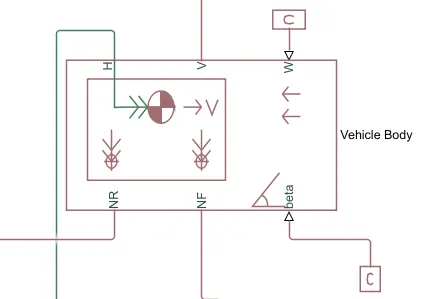
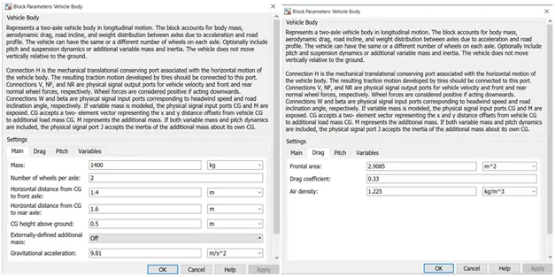
- Models the physical aspects of the vehicle body, including its mass, frontal area, and aerodynamic properties.
- Contains ports for connecting various components:
- H: Hub port used to connect the wheels to the main body of the vehicle.
- V: Output port for vehicle velocity.
- W: Input port for modeling wind velocity acting against the vehicle.
- NR: Output port to connect the rear wheels.
- NF: Output port to connect the front wheels.
- Beta: Input port for simulating hill climbing forces.
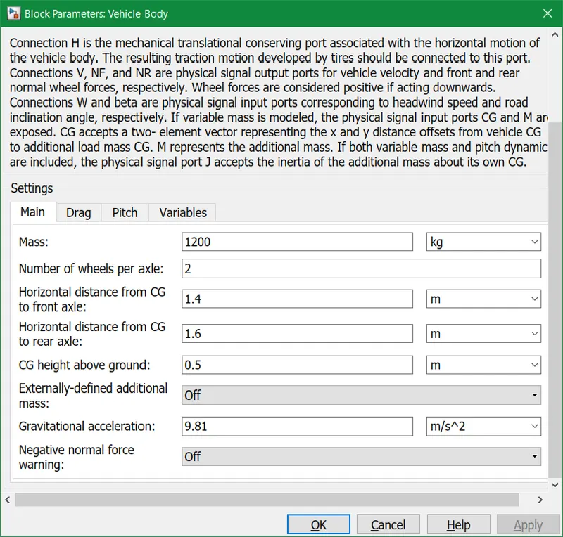
- Model parameters to set up mass, frontal area amd others.
Vehicle Body Subsystem:
- Integrates the vehicle body block, tire blocks, and gear block into a single subsystem.
- Four tires are connected, with the right two tires representing the rear wheels and the remaining two representing the front wheels.
- Rear axle is connected to the gear for rear-wheel drive configuration.
- Wind velocity and hill-climbing angle ports are connected to physical constant blocks set to zero.
Subsystem Connections:
- The mechanical input from the motor and controller block is fed into the gear block, which then influences the velocity of the vehicle body.
- Outputs the velocity at which the vehicle body moves, providing a visual representation of the vehicle's behavior during simulation.
Tire Block:
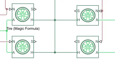
- Represents the tires of the vehicle.
- Allows customization of tire geometry, dynamics, rolling resistance, and other characteristics.
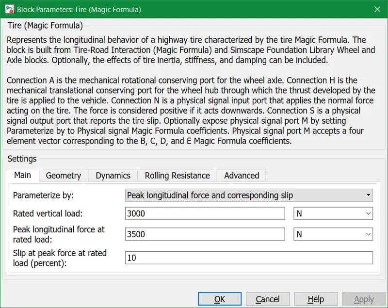
- Here we can also change the geometry , dynamics, rolling resistance other characteristics if we want
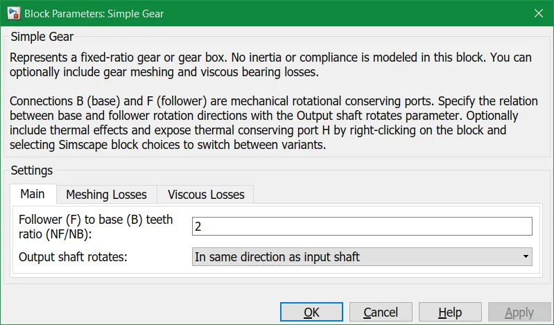
Simple Gear Block:
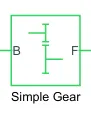
- Models a fixed gear system with no inertia effects.
- Parameters such as gear teeth meshing can be adjusted.
- Used to simulate the transmission system of the vehicle.
Motor and Controller Subsystem:
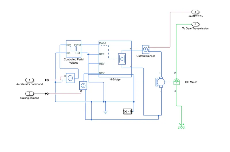
The Motor and Controller Subsystem plays a crucial role in the operation of the electric vehicle model. It consists of several key components designed to control the operation of the DC motor and regulate the power supplied to it. Below is a detailed explanation of each component:
DC Motor:
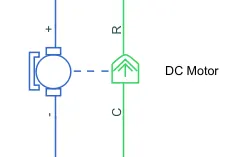
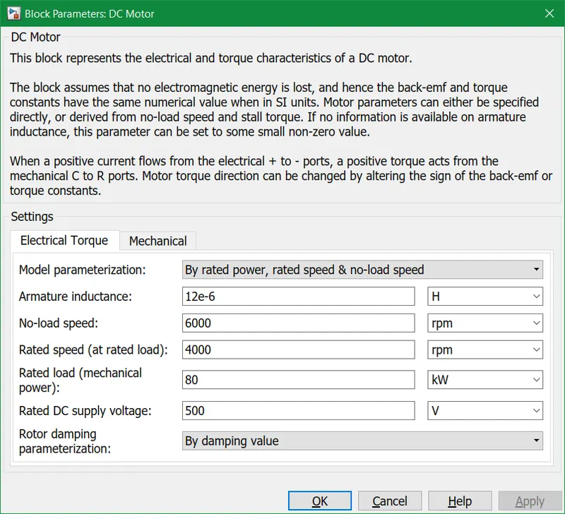
- The DC motor block is chosen for its simplicity and ease of modeling.
- Divided into mechanical and electrical sides.
- Mechanical side (right) has ports C (casing) and R (rotor) for torque generation.
- Electrical side (left) has positive and negative ports for voltage application.
- Parameters like rated power, rated speed, and no-load speed are set to customize the motor's behavior.
- C port is connected to the mechanical reference, while R port is connected to the gear in the vehicle body block.
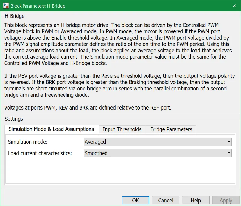
H-Bridge:
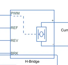
- Acts as a power converter, providing the necessary DC voltage from the battery to the DC motor.
- Consists of PWM (Pulse Width Modulation), reference, reverse, and brake ports.
- Configured in average simulation mode to expedite simulation time.
- Output voltage amplitude adjusted to 400 volts based on the DC motor requirements.
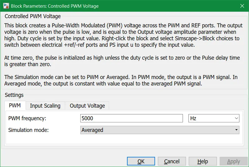
Controlled PWM Voltage:
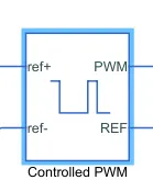
- Generates pulse width modulated voltage signals based on the duty cycle.
- Duty cycle determines the ratio of the time the switch is ON to the total cycle time.
- Parameters set to default values, and simulation mode chosen as averaged for quicker simulations.
Controlled Voltage Source:
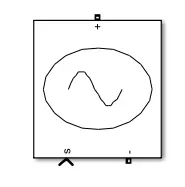
- Provides controlled voltage necessary to maintain the output voltage regardless of current.
- Used for both acceleration and deceleration.
- Electrical reference block creates grounding effect between components.
- Solver configuration block used to solve equations, particularly in connection with the REV port of the H-Bridge block.
Overall, the Motor and Controller Subsystem effectively manages the power flow and control signals to ensure the proper functioning of the electric vehicle model. It facilitates the conversion of electrical energy from the battery into mechanical energy for propulsion, allowing for accurate simulation and analysis of the vehicle's performance.
Battery Subsystem:
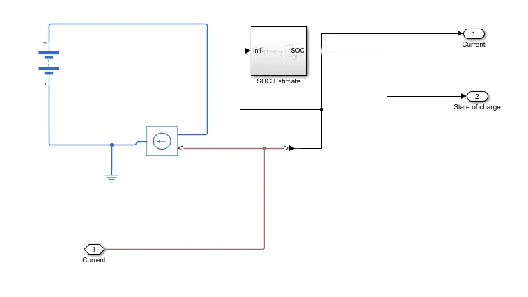
The Battery Subsystem serves as the energy storage unit for the electric vehicle (EV), storing electrical energy in DC form and supplying it for operation.
It consists of several key components designed to manage and regulate the flow of electrical energy. Here's a breakdown of each component:
Battery:
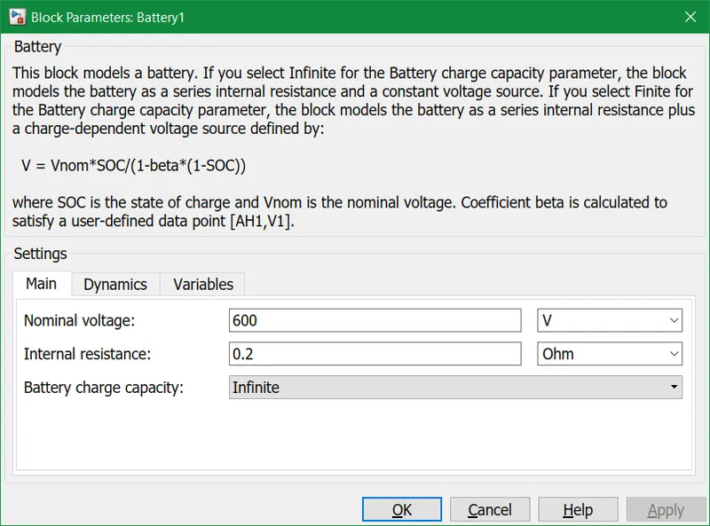
- Nominal voltage set to 600 volts, internal resistance set to 0.2 ohms, and infinite charging capacity.
- Designed to store electrical energy and provide it to the DC motor and H-bridge blocks.
- Nominal voltage is sufficient for supplying power to the motor and H-bridge.
Controlled Current Source:
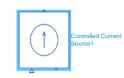
- Produces an ideal current to maintain a specified current regardless of voltage across it.
- Ensures a constant current flow within the battery subsystem.
Current Sensor:
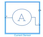
- Represents an ideal current sensor, measuring the current in the battery circuit and DC motor.
- Converts the measured current into a physical signal proportional to the current.
- Sends the signal to the controlled current source for further processing.
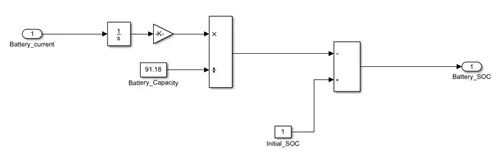
SOC (State of Charge) Estimate Subsystem:
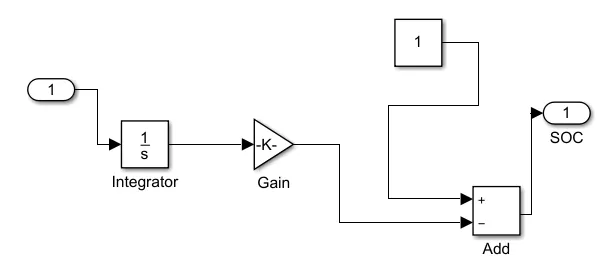
- Utilizes various blocks to estimate the state of charge of the battery.
- Integrator block integrates the current signal over time.
- Gain block adjusts the signal based on the battery's ampere-hour rating.
- Constant block ensures the battery is assumed to be fully charged.
- Sum block performs addition and subtraction operations.
- All blocks integrated into a subsystem called SOC estimate to estimate the battery's state of charge.
- Scope block used to plot the output current signal from the battery for visualization.
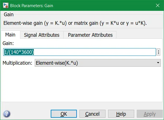
Speed Measurement:
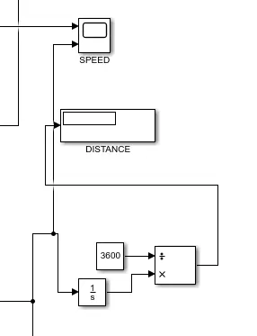
- Modified scope block used to measure the speed by comparing the vehicle's velocity output with the reference velocity from the drive cycle.
- Allows for monitoring and comparison of vehicle speeds.
Distance Measurement:
- Utilizes mathematical blocks and scope block to measure the distance traveled by the vehicle.
- Integrator block integrates the velocity signal over time.
- Dividen block divides the integrated speed by a constant to obtain distance traveled in kilometers.
Longitudinal Driver and Drive Cycle:
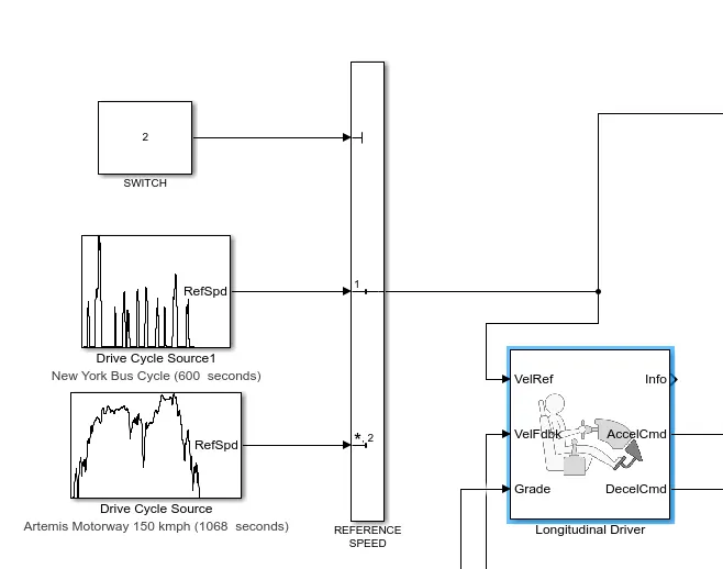
- Longitudinal driver block generates normalized acceleration and deceleration commands based on reference and feedback velocities.
- Reference velocity comes from the drive cycle source, while feedback velocity comes from the vehicle's body.
- Comparison between reference and feedback velocities determines acceleration or deceleration commands.
- Simulink-PS converter block converts logic data into voltage signals for acceleration and deceleration commands.
- Ports include Velref (reference velocity), Velfdbl (feedback velocity), Grade (grade or inclination angle), Info (bus signals), Accelcmd (acceleration command), and Deacclcmd (deceleration command).
Drive Cycle:
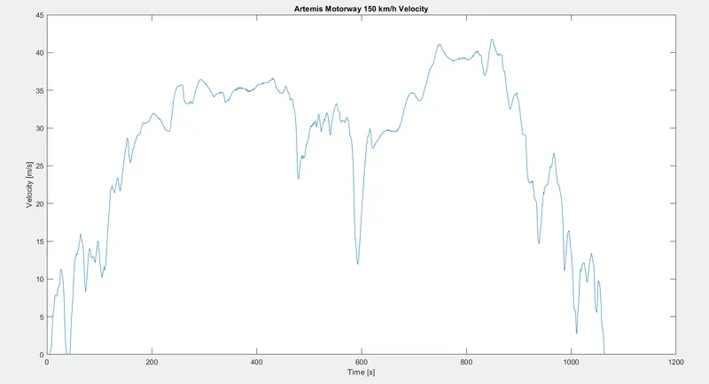
A drive cycle is a dataset that records the velocity and time data, representing the vehicle's motion. It typically mirrors real-world driving conditions and is essential for modeling vehicle behavior accurately. In this project, two drive cycles were utilized: the "New York Bus Cycle" and the "Artemis Motorway of 150 km/h." Drive cycles serve various testing purposes, including mileage, pollution tests, and acceleration and top speed evaluations.
Block Parameters:
The Artemis Motorway 150 km/h drive cycle graph was input into the vehicle model. This data provides the velocity profile for the vehicle's operation.
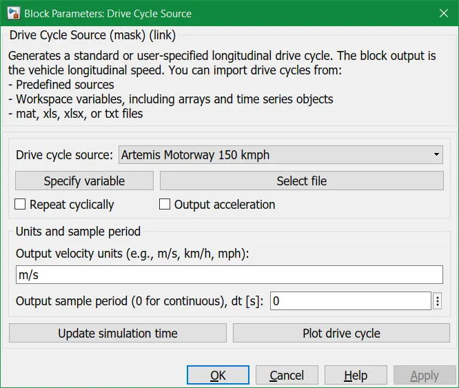
Artemis Motorway 150kmph Drive cycle graph is given as input to the vehicle model:
Results:
After running the drive cycle for the electric vehicle (EV) model, outputs from speed, current, and state of charge (SOC) scopes were collected. The distance traveled by the vehicle during the drive cycle was also measured using a display block. The simulation runtime was adjusted to match the duration of the drive cycle, which was 1068 seconds.
Speed Scope:
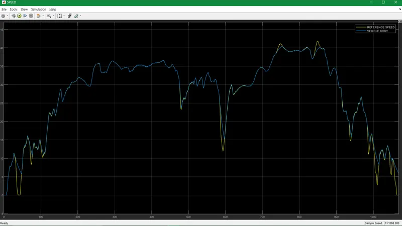
The speed scope displays two signals: the blue signal represents the vehicle's actual speed, while the yellow signal represents the Artemis drive cycle data. The longitudinal driver successfully maintains the vehicle's speed according to the reference speed provided by the drive cycle data. The graph effectively overlaps during acceleration and deceleration phases.
Current Scope:
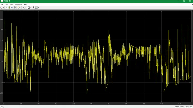
The current scope illustrates how the current flowing from the battery to the motor varies throughout the drive cycle. This information is crucial for monitoring power consumption and ensuring the battery operates within its limits.
SOC Scope:
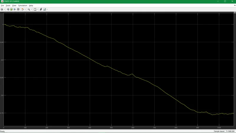
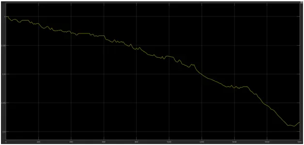
The SOC scope depicts the variation in the battery's state of charge over the duration of the drive cycle. The battery model begins with an SOC of 100%, and as the simulation progresses, the SOC decreases. Notably, during braking periods, regenerative braking replenishes the battery charge, resulting in an uplift in the SOC graph. At the end of the simulation, the SOC stabilizes at around 75%.
Battery Parameters:
The nominal voltage of the battery is set to 460V, consistent with the motor's rated voltage. The battery's specifications are derived from Table 3 data, providing critical information for modeling its behavior accurately.
Battery SOC Estimation:
To estimate the state of charge of the battery, the Coulomb counting method is employed. This method subtracts the charge taken from the battery from the initial SOC. The equation for SOC estimation is modeled in Simulink to track the battery's state throughout the drive cycle.
Vehicle Model:
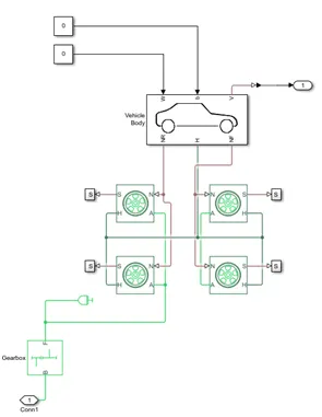
The vehicle model subsystem encompasses the vehicle body, tire, and gear blocks. These components work together to simulate the vehicle's motion and performance accurately.
Vehicle Dynamics:
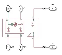
The Vehicle Body block represents a two-axle vehicle body with adjustable mass, geometry, and drag properties, facilitating longitudinal motion. It accounts for mass, aerodynamic drag, road incline, and weight distribution between axles during acceleration and road profile changes. This block, sourced from Simscape/Driveline/Tires & Vehicles library, is configured based on parameters such as mass, frontal area, and drag coefficient, sourced from Table 1, TATA NEXON specifications.
Tire Modeling:
The Tire (Magic Formula) block models tire longitudinal behavior using the Magic Formula, employing four fitting coefficients. It accurately captures tire dynamics under various pavement conditions. Load-dependent magic formula coefficients are chosen for this project. The tire parameters, including inertia and rolling radius, are sourced from Table 1, TATA NEXON specifications.
Gear Transmission:
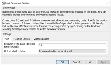
The Simple Gear block simulates a gearbox, constraining base and follower gears to co-rotate with an adjustable gear ratio. It offers options for friction losses and fault triggering. This block, accessed from Simscape/Driveline/Gears library, provides precise control over gear behavior in the driveline.
Simulation Results:
The distance covered by the vehicle in WLTP Class 3 drive cycle is 23.27km:
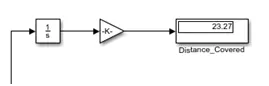
The vehicle's performance during the Artemis Motorway 150 km/h drive cycle is analyzed. Integration of vehicle velocity provides the distance covered, revealing a total of 23.27 km traveled. The comparison between drive cycle speed and vehicle speed indicates alignment, with minor deviations observed during sudden braking, attributed to tire inertia.
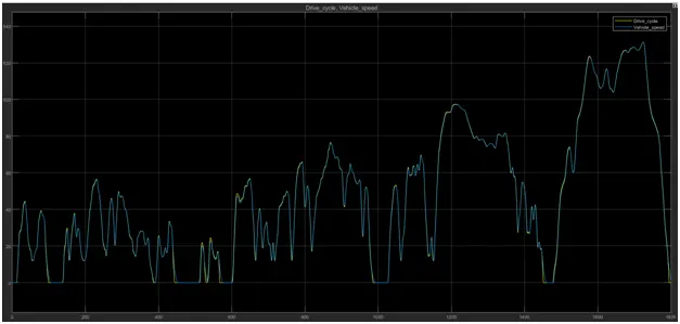
The above figure shows the drive cycle speed and vehicle speed plot. We can see that vehicle follows drive cycle in all regions. Slight variations in the curve are in the regions of sudden braking. This may be due to the inertia of the tires.
Acceleration and Deceleration:
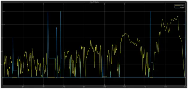
The longitudinal driver generates acceleration and brake signals, crucial for controlling the vehicle's motion. The plot illustrates the commands issued during acceleration and deceleration phases.
PWM Signal Analysis:
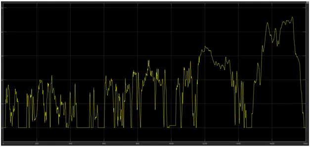
The PWM signal to the H-Bridge varies with speed requirements, reaching maximum magnitude during acceleration and zero during braking.
Battery State of Charge (SOC):
The SOC plot demonstrates battery discharge during acceleration and recharge during regenerative braking. By the end of the simulation, the SOC stabilizes at 82%, indicating efficient energy management.
Results:
The EV model was subjected to the specified drive cycle, and outputs from speed, current, and SOC scopes were analyzed. Additionally, the distance covered by the vehicle during the drive cycle was measured using the display block. Before initiating the simulation, the runtime was adjusted to match the drive cycle duration of 1068 seconds.
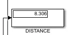
From the simulation results obtained, the distance traveled by the vehicle was determined to be 8.306 kilometers within the 1068-second simulation period. Furthermore, the analysis revealed that the battery charge remained at 75% by the end of the simulation.
This outcome provides valuable insights into the vehicle's performance, indicating its capability to cover a significant distance while maintaining a substantial portion of its battery charge. Such findings contribute to the overall assessment of the EV model's efficiency and suitability for real-world applications.
Google drive link of model: Click here
Conclusion:
In conclusion, the project on the design of an electric vehicle (EV) using MATLAB and Simulink has provided valuable insights into the intricacies of electric vehicle engineering and simulation. Through this endeavor, several critical aspects of EV design, simulation, and analysis have been explored and understood.
The constructed MATLAB model, incorporating components such as the vehicle body, battery, motor, controller subsystems, and drive cycle analysis, accurately captures the dynamics and performance of an electric vehicle. Simulation results from various scopes and subsystems, including speed, current, SOC, and distance measurements, offer a comprehensive overview of the EV's behavior under different conditions.
Analysis of the simulation outcomes indicates that the EV model adheres well to the specified drive cycle, with efficient energy utilization and appropriate vehicle performance. Integration of regenerative braking enhances battery charging efficiency, contributing to sustainable energy management.
Furthermore, the project underscores the importance of design optimization, considering factors like motor selection, battery capacity calculations, and efficiency improvements to meet performance requirements while minimizing costs and energy consumption. Real-world application considerations, such as cost, size, weight, and efficiency trade-offs, have been taken into account throughout the design process.
Overall, the project serves as a testament to the capabilities of MATLAB and Simulink in modeling complex systems like electric vehicles and analyzing their performance. The insights gained from this project are invaluable for future endeavors in electric vehicle design, development, and deployment, contributing to the ongoing evolution of sustainable transportation solutions.
MATLAB Model Summary:
The MATLAB model incorporates driver, vehicle, and motor parameters, with design considerations based on equations and data analysis. Motor and battery ratings are selected based on datasheet information and model calculations. Analysis of vehicle velocity and battery SOC further validates the model's accuracy and effectiveness. The model file (.slx) is provided for reference and further analysis.
Google drive link of model: Click here
Key Learnings from the Project:
1. Electric Vehicle (EV) Basics:
Understanding the fundamental principles of electric vehicles, including their reliance on electric motors for propulsion, the significance of batteries, and the differences in power delivery compared to internal combustion engines.
2. Powertrain Design Considerations:
Learning the factors involved in designing an electric vehicle powertrain, such as motor ratings, battery capacity, energy consumption, and range estimation.
3. Drive Cycle Analysis:
Familiarity with different drive cycles used for testing and simulation, such as the WLTP Class 3 cycle, and how to interpret drive cycle data to assess vehicle performance and energy consumption.
4. Component Modeling in Simulink:
Hands-on experience with modeling various vehicle components using Simulink, including the vehicle body, tires, gears, battery, motor, and controller subsystems.
5. Integration of Subsystems:
Understanding how different subsystems interact within the vehicle model and how to properly integrate them to simulate realistic vehicle behavior.
6. Battery Management and SOC Estimation:
Learning about battery management systems, state of charge (SOC) estimation methods, and how to implement them in Simulink for monitoring and managing battery performance.
7. Simulation Analysis:
Gaining proficiency in analyzing simulation results from speed, current, and SOC scopes to evaluate vehicle performance, energy efficiency, and battery utilization.
8. Design Optimization:
Exploring strategies for optimizing vehicle design, including motor selection, battery capacity calculations, and efficiency improvements to meet performance requirements while minimizing costs and energy consumption.
9. Regenerative Braking:
Understanding the concept of regenerative braking and its importance in electric vehicles for recovering energy during deceleration and improving overall efficiency.
10. Real-World Application Considerations:
Considering real-world factors such as cost, size, weight, and efficiency trade-offs when selecting components and designing electric vehicle systems.
These key learnings provide a comprehensive understanding of electric vehicle design principles, simulation techniques, and performance evaluation, essential for future projects and applications in the field of electric mobility.