Final Project: Design of an Electric Vehicle

 Aim:-

Create a MATLAB model of electric car which uses a battery and a DC motor. Choose suitable blocks from Powertrain block set. Prepare a report about your model including following.

Objectives:-

       1. System level configurations

       2. Model parameters

       3. Results

       4. Conclusion

 Theory:-

An Electric Vehicle (EV) is a vehicle that uses one or more electric motors or traction motors for propulsion. An electric vehicle may be powered through a collector system by electricity from off-vehicle sources, or may be self-contained with a battery, solar panels, fuel cells or an electric generator to convert fuel to electricity. EVs include, but are not limited to, road and rail vehicles, surface and underwater vessels, electric aircraft and electric spacecraft.

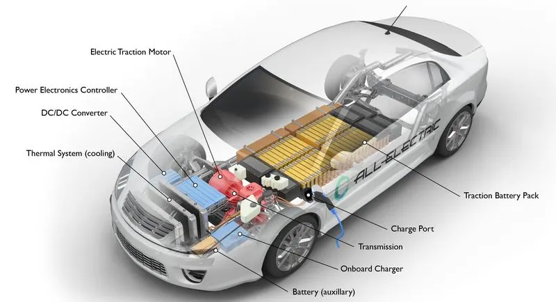
Components of an EV :- 

• EVs have no need for the fuel engine and gear transmission, the two of the most crucial components for internal combustion vehicles.
• An electric powered car has three primary components - Battery, motor controller, and the electric motor.

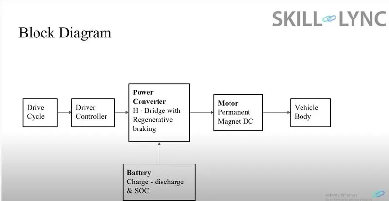
Components :-

The main components of an EV are:-

• batteries
• power converters
• motor controllers
• motor/generator
• transmission system
• wheels/tires

1. Battery :- The battery of an electric car can be charged through the use of ordinary grid electricity at a specialized power station. But aside from the conventional lithium-ion battery technologies, there are also other major battery technologies which can be used for electric cars.

• Lithium-Ion Batteries :- This battery technology gives extra performance and range. However, it also carries the highest price tag. Lithium-ion batteries are lighter than Lead acid and Nickel metal. These are also the batteries used in digital cameras and smartphones.
• Lead Acid Batteries :- This battery technology is the most popular. It is also the cheapest among the battery technologies. What’s good about it is it’s 97% recyclable.
• Nickel Metal Hydride Batteries :- This battery technology provides higher output and better performance but it costs much more than lead-acid batteries.

     2. Motor Controller :- 

• The motor controller of an electric car administers its complete operation and the distribution of its power at any given moment. It acts as a floodgate between the motor and batteries. It helps monitor and regulates all key performance indications such as the vehicle’s operator, motor, battery, and accelerator pedal.
• . It has a microprocessor which can limit or redirect current. It is used to either improve the mechanical performance of the car or suit the operator’s driving style. There are also more refined controllers which are capable of greater accuracy and thus, higher efficiency.

     3. Electric Motor :-

• Unlike a gasoline engine with lots of moving parts, a motor only has one moving part. This makes it a very reliable source of motive power. Choosing an electric motor depends on the car’s system voltage. 
• They can be structured to use either AC or DC current. AC motors are less expensive and lighter compared to DC motors.
• They are also more common and they tend to suffer from less mechanical wear and tear. However, AC technology requires a more refined or sophisticated motor controller.

     4. power Controller :- 

• Power converters convert the power coming from the battery to a usable form for the motor.
• This conversion can be from DC to AC or vice versa and can even be between 2 different magnitudes of DC to DC or AC to AC. 

     5. transmission system :- 

• The transmission system is needed for the vehicle to change speeds as it accelerates/decelerates.

     6. wheels/tires :-

• The wheels are needed for traction on the roads and depending on the powertrain, the EV may be an FWD or RWD (forward or rear wheel drive). 
•  If a vehicle is an FWD, only the front axle wheels produce propulsion i.e.. rotate from motor effect and if it is an RWD, the back axle wheels produce it instead. All wheel drives (AWDs) also exist where the front and rear axle wheels work together to produce propulsion. 

System Level Configuration :- 

To model an EV in SIMULINK, we will need to model the aforementioned components separately and then have them work together. All the main components are available in the library of SIMULINK blocks and we will be adding each component and configuring its parameters to fit the requirements of the model. First, I have modelled the vehicle main body. 

Vehicle Body :-

To model a vehicle's body, we need to first add the vehicle body block and this is shown below:-

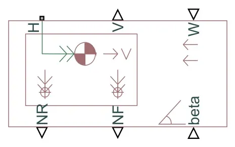
This block contains 6 ports which can be used to model the various aspects of the vehicle body. The ports are mentioned and elaborated below:-

• H - This stands for 'Hub' and is used to connect the hubs of the wheels to the main body of the vehicle.
• V - This is a physical signal output port which stands for 'Velocity' and is used to output the speed/velocity at which the vehicle is moving at. 
• W - This is a physical signal input port and allows us to model a 'headwind' acting on the vehicle by giving a speed for it.
• NR - This is a physical signal output port to model the rear wheel normal forces. 
• NF - This is a physical signal output to model the front wheel normal forces. 
• beta - This is a physical signal input port and allows us to model the vehicle on an inclination angle to create the effect of a hill climbing force.

If we double click the vehicle body block, we can see and modify its parameters and this is shown in the image below:-

 

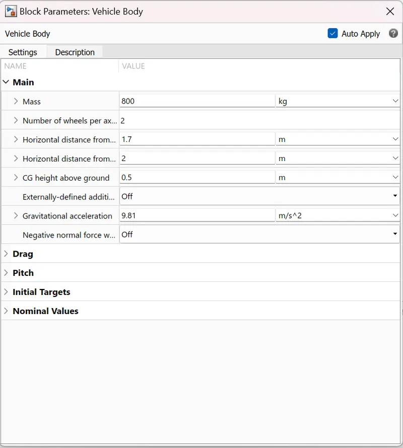
We can see from this image that the parameters of frontal area, drag coefficient and air density can be modified in order to effect the drag force acting on the vehicle. In my case, I have only changed the drag coefficient to 0.3 from the default value 0.4 in order for the model to resemble a typical sedan. Air density and frontal area are normal for this type of vehicle. 

Tries :-

• The tires used in this EV model are the 'magic formula' tires. There are several tire blocks that can be used for modelling a vehicle but I have used the magic formula ones because it allows us to model the longitudinal behavior of vehicle tires on highways.
• They also allow us to model extra effects such as tire inertia, stiffness which allow for greater accuracy of real world conditions. 
• The magic formula tire block is shown below:-

 

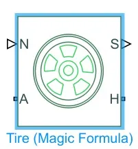
We can see that it has 4 ports and they are :-

• N - This port stands for 'Normal' and is the physical signal input port for the normal force acting on the tire and is considered positive in the downwards direction.
• S - This port stands for 'Slip' and is the physical signal output port is that reports the slip acting on the tire.
• A - This port stands for 'Axle' and is the mechanical rotational conserving port for the wheel axle. 
• H - This port stands for 'Hub' and is the mechanical translational conserving port for the wheel hub through which the thrust developed by the tires is applied to the vehicle body.

Double clicking the magic formula tire block takes us to its parameters :-

Main:-

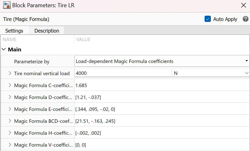
As we can see, we are parameterizing the tires with 'Load dependent Magic Formula coefficients' and the remaining parameters that follow with it are default. 

Geometry:- 

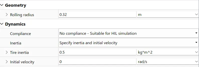
The image below shows the parameters of the tire geometry. There is only one parameter that can be modified and it is the rolling radius and has been set to a nominal value of 0.32m.

Dynamics :- 

The next parameters are the dynamics of the magic formula tires. This is where we can model additional effects e.g. tire inertia and the initial velocity if we are modeling to specify those 2 conditions. 

Rolling Resistance :-

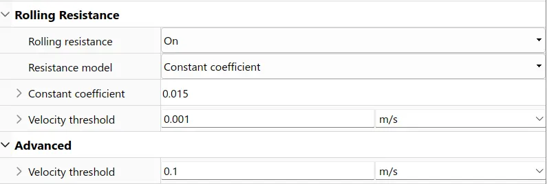
Here, we can model the rolling resistance parameters on the tires and I have chosen to switch ON the rolling resistance force on the tires. Also, I have selected a constant coefficient of rolling resistance of 0.015 and a velocity threshold of (1e^-3).

Advanced :-

Finally, the last parameter for the magic formula tires is the velocity threshold and this has been set to 0.1m/s. Below this speed, the block will not model any of the aforementioned effects of motion on to the tire, hence called a 'threshold' velocity. 

Gear :-

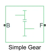
Next, we will model the transmission system of the EV. I have decided to use a 'Simple Gear' block so as to simplify the transmission system parameters. This block models a gear system with a fixed gear ratio with no inertia effects, however we can modify the effects of the meshing of the gear teeth. The simple gear block is shown below:-

Double clicking the simple gear block takes us to its parameters :-

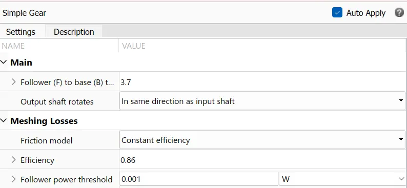
Main :-

The main parameters of the simple gear are the follower to base teeth ratio and this has been set to 3.7. I have also specified that the output shaft rotates in the same direction as the input shaft as opposed to the opposite direction of the input shaft. 

Meshing Losses :-

The meshing losses I have selected follow a constant efficiency friction model with an efficiency of 0.86 and follower power threshold of 0.001W. 

Side Shaft :-

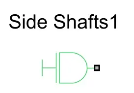
An inertia block has been added to the workspace to provide an ideal mechanical rotational inertia for the simple gear block. This block has only one mechanical rotational conserving port and the positive direction of the block is from the port to the reference point which would be the simple gear in this case. The inertia torque acts in the positive direction is the inertia is accelerated in the positive direction. The inertia block is shown below:-

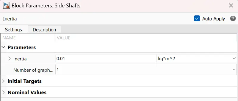
The inertia block parameters only allow for us to modify the inertia and this parameter has been kept at the default value of 0.01. 

Wind and Slope :-

• As mentioned earlier, the velocity block allows us to model the effects of wind resistance and road inclination through the 'W' and 'beta' ports respectively.
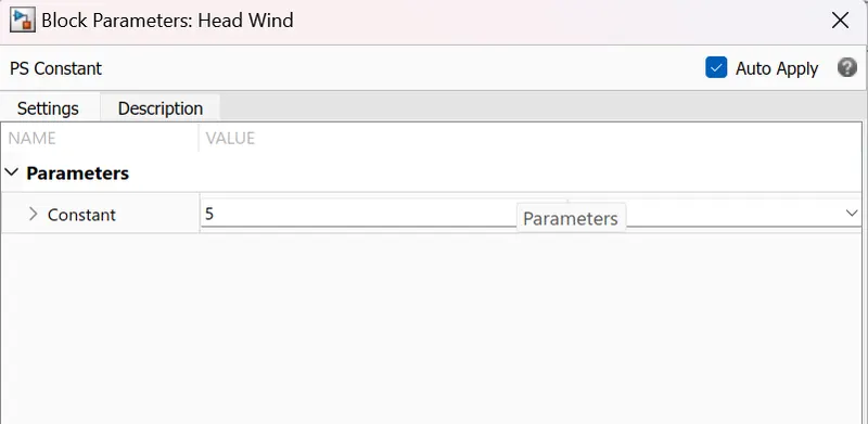
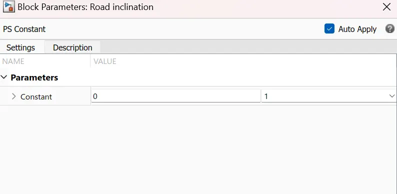
• In my model, I have used a 'PS - Constant' block to model the parameters of wind and road inclination on the vehicle's motion.
• For the wind effect, I have given a constant signal of 5m/s and this acts in the opposite direction to the direction of motion i.e.. headwind. For the road inclination, I have given a constant signal of 0.
•  The block parameters of the wind and slope effects are shown in the images below:-

Velocity Subsystem :-

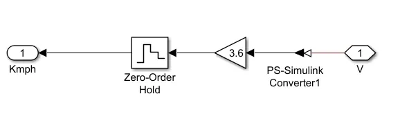
The velocity port which outputs the velocity signal of the vehicle body block has been modified. By default, the velocity signal that is output from the vehicle body block is measured in miles per hour. To change these units, I have implemented a small subsystem from the output of the velocity port. This subsystem uses the following blocks:-

• PS - Simulink converter - this block will convert the physical signal of velocity to a logic signal.
• Gain - This block uses a multiplication factor of 3.6 to convert the miles per hour units to kilometres per hour.
• Zero - Order Hold - This block is used implement a zero order hold sample period.

The inside of the subsystem is shown below:-

Vehicle Body Subsystem :-

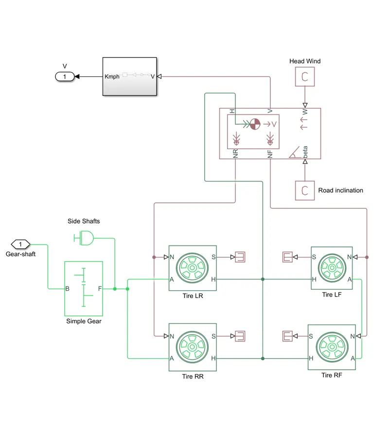
• As seen in the diagram above, the various blocks are connected to model the vehicle body. 4 magic formula tire blocks are used as the vehicle will have 4 tires, 2 on each axle. The tires are LR, LF, RR and RF (left rear, left front, right rear, and right front).
• The normal ports of each tire are connected to the appropriate NR and NF ports on the vehicle body block.
• The hubs of each tire are connected together and an extra connection is made from them to the vehicle body block.
•  The wind velocity and road incline are provided with constant physical signals of 5m/s and 0 degrees respectively.
• The velocity port has been connected to the velocity subsystem and the connection from the subsystem is open to the 'v' port. 
•  The base port of the simple gear has been left open to the 'Gear-Shaft' port to take in a rotational signal. 

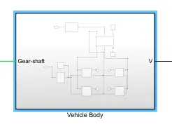
This subsystem is created so that less space is taken up in the workspace and now, we only need the open ended connections to be modified. 

Motor :-

For the EV model, I have selected to use a DC motor block as the motor. This is because DC motors are easier to model and have fewer parameters to modify for a particular application. For this model, a DC motor will do just fine. The DC motor block is shown below:-

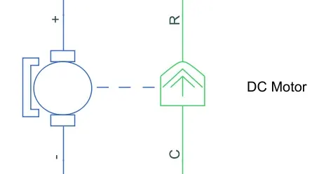
• As we can see, there are 2 sides to the block: the mechanical side on the right and the electrical side on the left. 
• The mechanical side has 2 ports, C and R. The C refers to the casing and the R for the rotation of the rotor which produces a torque. 
• The electrical side has a positive and a negative terminal for the voltages to be applied. If a positive voltage is applied to the DC motor block from the positive to the negative terminal, a positive torque will act from the C port to the R port. 
• The direction of the torque produced by the DC motor can be changed by changing the sign of the back emf or the torque constant. 
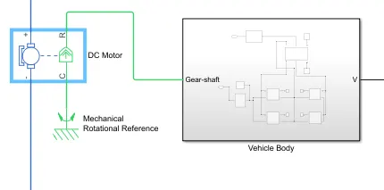
• The C port of the mechanical side needs to be connected to a mechanical rotational reference because it will be stationary. 
•  The R port will be connected to the open connection of the simple gear from the vehicle body block. 
• The positive terminal on the electrical side is connected to the positive terminal of a power converter which in my case will be an 'H bridge'.

The mechanical rotational reference block is shown below:-

 

Double clicking the DC motor block takes us to its parameters. The electrical torque parameters are first considered. Here, I have chosen to parameterize the block 'By rated power, rated speed & no-load speed'. This lets us modify parameters such as DC supply voltage, rated load. I have kept all values default except for the no load speed, rated speed, rated load and the DC supply voltage which were changed to the values shown in the image below:-

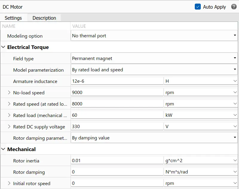
In the above mechanical parameters, we can modify the rotor inertia, damping and initial rotor speed. However, these values were kept to their default settings.

Once the DC motor block has been parameterized, the following connections need to be made:-

 

Power Converter :-

The power converter is needed to provide power of the correct form and magnitude from one component to another. In the case of EVs, a power converter is needed to provide a DC voltage from the battery of the EV to the DC motor so that it can operate properly with the required parameters. As mentioned earlier, I have used an H-Bridge motor drive as my power converter. Its block is shown below:-

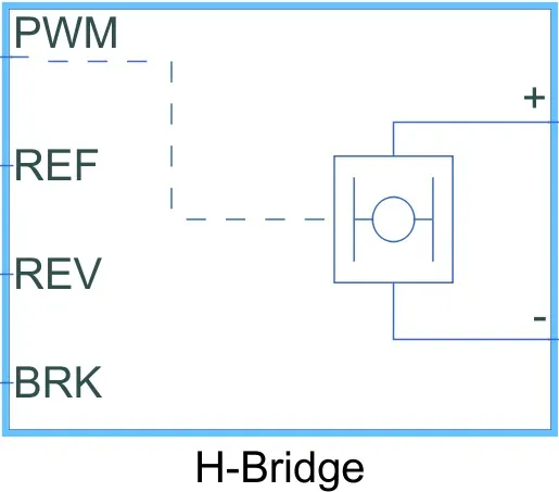
• The H Bridge has 2 sides to it: the left side is for the controlling of the voltage signals and the right side is for the terminals to provide the controlled voltage to the DC motor. The left side ports of the H-Bridge block are:-
• PWM - This stands for Pulse Width Modulation which will provide the voltage pulses to the H-Bridge either in the PWM or average mode.
• REF - This stands for Reference.
• REV - This stands for Reverse. 
• BRK - This stands for Brake. 

Opening the H-Bridge block will take us to its parameters shown below:-

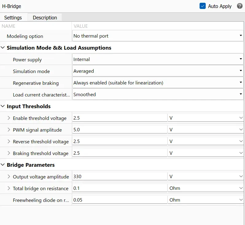
• The main parameters are for the simulation mode and load assumptions of the H-Bridge. I have selected the H-Bridge to run on an internal power supply with an averaged simulation mode instead of the PWM mode. 
• This is because using the PWM mode will result in significantly longer simulation times compared to using the averaged mode. 
• I have enabled the regenerative braking mode and set the load current characteristics to the smoothed option. 

• The next parameters of the H-Bridge are its input thresholds. Here we can set the various voltage limits of its 4 left hand side ports. These values are left to their default settings. 

• The last parameters for the H-Bride pertain to its bridge parameters. Only the first parameter of 'Output voltage amplitude' was modified. This is because the DC motor has been parameterized to run on a DC supply voltage of 330V. So this same value is used for the output voltage amplitude. 
• Once these parameters have been applied, close the parameter settings. The connections for this block will be made later on. 

Controlled PWM Voltage :-

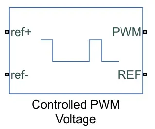
• I have used a 'Controlled PWM Voltage' block to provide a controlled pulse width modulated voltage to the H-Bridge block.
• The block will output the PWM voltage through its 'PWM' and 'REF' ports which will feed in to the same ports found on the H-Bridge block. If the pulse is low the output voltage is considered 0V whereas if the pulse is high, the output voltage will be equal to the output voltage amplitude which was set to 330V in the H-Bridge block.
• The pulses of voltage created by this block are dependent on the duty cycle which is the ratio of the time that the switch is ON to the time taken for 1 cycle (which is the time for which the switch is ON and OFF). The duty cycle is set by the input of the controlled PWM voltage block. 
• The duty cycle formula is given by:-
• Duty Cycle = (Ton/Tcycle)

where,

Ton = time ON

Tcycle = time taken for 1 cycle.

The block parameters are shown in the image below:-

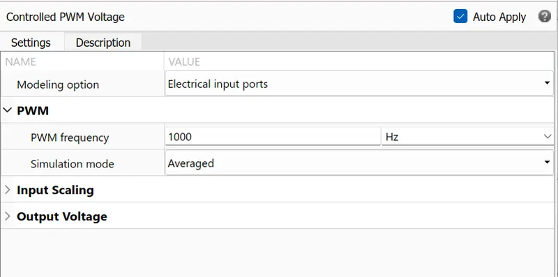
• The main settings pertain to the PWM parameters. Here all the parameters are maintained at their default values. I have chosen the 'Averaged' simulation mode so that the average value of the voltage pulses are generated and fed in to the H-Bridge.
• This will allow for quicker simulation times, just like for the H-Bridge block parameters. The remaining parameters of 'Input Scaling' and 'Output Voltage' are unchanged. 
• If these parameters have been applied, close the block parameter window. The connections for this block will be made later on. 

Controlled Voltage Source :-

• The input ports of the controlled PWM voltage block are still unconnected and that is because they require a controlled voltage source to provide the voltages to produce the voltage pulses to be fed in to the H-Bridge. 
•  For this, I have used the controlled voltage source block. This block is useful because it will provide the necessary voltage that is powerful enough to maintain the voltage at the output regardless of the current that passes through it. 

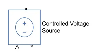
• In this model, 2 controlled voltage sources have been used. One block is to provide the voltage for the acceleration of the vehicle and the other is to provide the voltage for the deceleration of the vehicle. 

Electrical Reference :-

• The electrical reference block is used to create a grounding effect for electrical circuits. Any model that uses electrical or electronics components will need to have at least one electrical reference block in it.

• In my EV model, we are using this block for 2 occasions. The first is for to create an electrical ground between the controlled voltage source, controlled PWM voltage and the H-Bridge blocks. The second is for the battery system which will be modelled afterwards. 

Solver Configuration :-

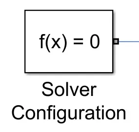
• The solver configuration block is used to solve any necessary equations in a model and in my case, I have used them in the connection to the 'REV' port of the H-Bridge block. The solver configuration block is shown below:-

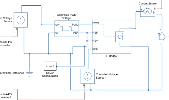
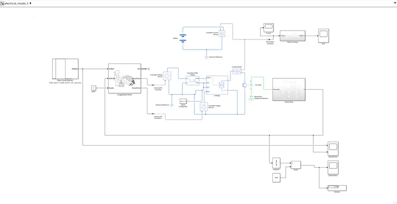
The image below shows the connections that can be made with the components discussed till this point. 

Longitudinal Driver :-

The longitudinal driver block is used for giving normalized acceleration and deceleration commands to a controller based on 2 sets of data. The first data set is the reference velocity and the second data set is the feedback velocity. The longitudinal driver block is shown below:-

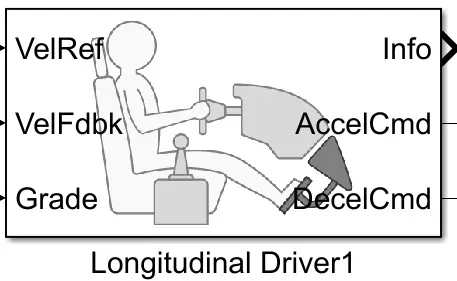
The longitudinal driver block has the following ports:-

• VelRef - This stands for the reference velocity and it is the velocity data provided from a drive cycle source.
• VelFdbk - This stands for the feedback velocity and it is the velocity data provided from the vehicle body's velocity port which outputs the velocity data. 
• Grade - This port provides a grade or inclination angle for the surface on which the vehicle is travelling in degrees. 
• Info - This port is for the bus signals which consist of block calculations e.g. acceleration/deceleration command, difference between reference and vehicle speed. 
• AccelCmd - This port provides the acceleration command to a controlled voltage source. 
• DecelCmd - This port provides the deceleration command to another controlled voltage source. 

• The working of the longitudinal driver block is simple. The reference velocity data coming from a drive cycle source is compared to the feedback velocity data coming from the vehicle body block.
•  If the reference velocity is greater than the feedback velocity, an acceleration command will be given as an output to the controlled voltage source.
•  If the reference velocity is lesser than the feedback velocity, a deceleration command is given as the output to another controlled voltage source instead. For the acceleration and deceleration commands to be given as output signals.
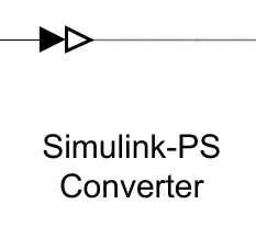
•  I have used a Simulink - PS converter block. This block is needed whenever we wish to connect a Simulink input signal to a physical signal. In this case, the input signal is velocity data and this is logic data which we want to convert to a physical signal i.e.. voltages to the controlled voltage source. 

The Simulink - PS converter block is shown below:-

The longitudinal driver block parameters are shown in the image below:-

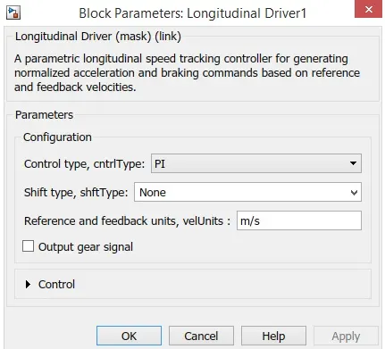
As we can see, I am using a PI controller for this block and I have set the reference and feedback velocities to be in m/s units. All the other parameters are unchanged. 

Grade :-

The grade port of the longitudinal driver block is connected to a constant block with a constant value of 0. This is so that no road inclination is modelled for the simulation.

Drive Cycle :-

 I have used an industry standard 'WOT' drive cycle. This drive cycle stands for 'Wide Open Throttle' and it models the situation where the vehicle is made to accelerate at full power and maintained at a particular speed and made to decelerate back to rest. 

When the 'WOT' drive cycle is chosen, some extra parameters are made available for modification which are shown below:-

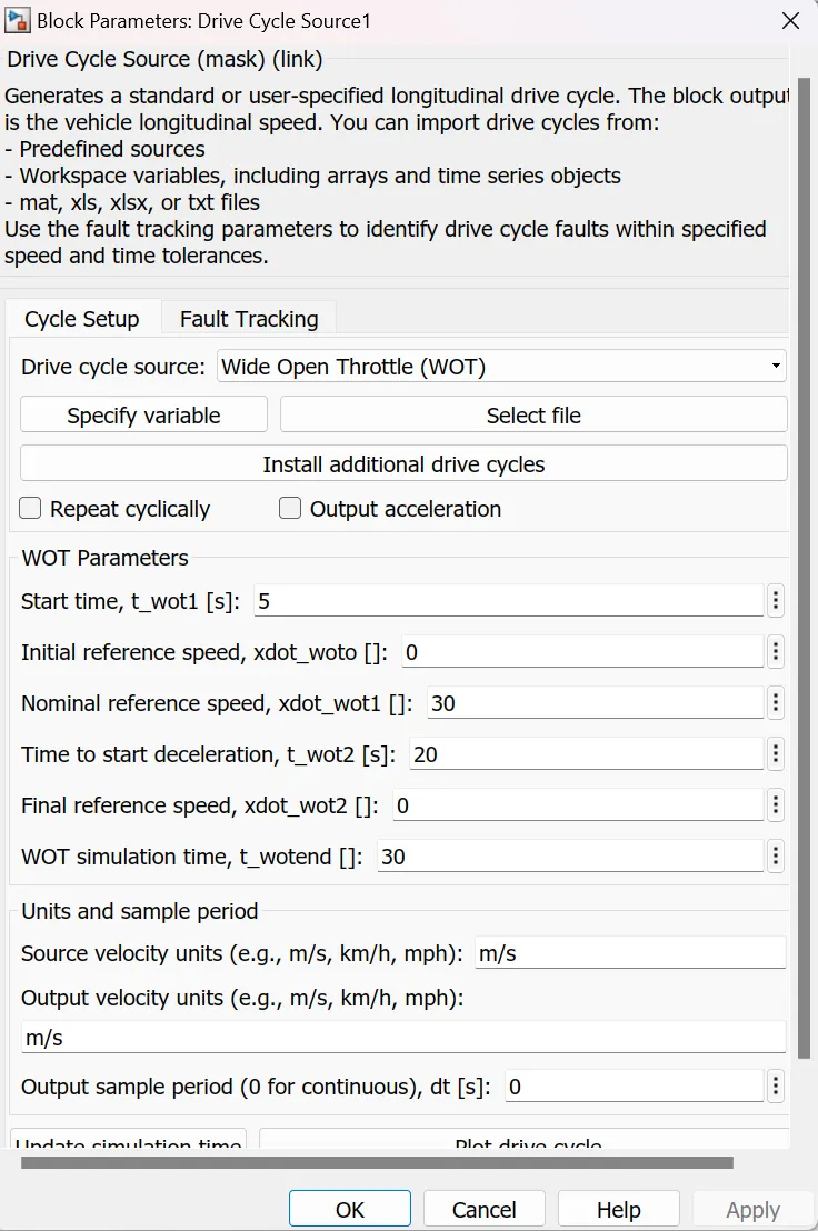
• As we can see, with the 'WOT' drive cycle, we can modify the start time, time to start deceleration and the entire duration of the drive cycle.
• I have used a start time of 5 seconds meaning that the vehicle will begin acceleration after 5 seconds of starting simulation.
• I have used a nominal reference speed of 30m/s and this refers to the maximum speed the vehicle should achieve.
• I have set the deceleration to begin at t = 20 seconds and the whole cycle is set for a duration of 30 seconds.
• The input and output velocity units are both set to m/s. 

The plot below shows the custom WOT drive cycle I have created. 

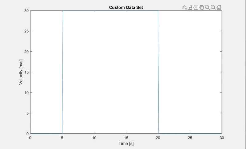
Once the drive cycle parameters have been set as shown above, the output port of the drive cycle can be connected to the reference speed port of the longitudinal driver block. If all the parameters have been set as discussed, the connections can be made as shown in the image below:-

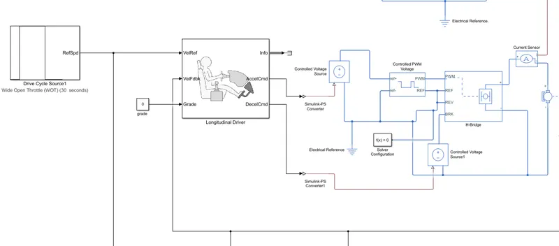
The connection for the vehicle feedback is left open ended for now and will be connected later on. Next, we can model the battery of the EV. 

Battery :-

The battery will be the energy store of the EV and will contain the electrical energy in DC form and provide this energy to the DC motor for it to operate. The battery block used is a simple one and considers only the basic parameters. 

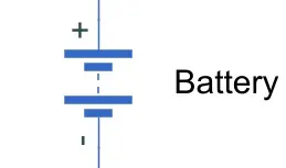
The battery block parameters are shown below:-

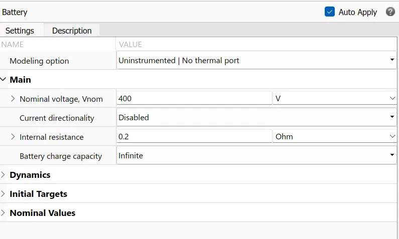
As we can see, the battery block parameters include the nominal voltage, the internal resistance and the battery charge capacity. I have used a nominal voltage of 400V, an internal resistance of 0.2 Ohms and an infinite battery charge capacity. The nominal voltage is selected so that it is more than sufficient to supply the voltage to the DC motor and the H-Bridge blocks. 

Controlled Current Source :-

The controlled current source block is a part of the battery system used in the EV model. Similar to the controlled voltage source, this block will represent an ideal current source that is powerful enough to maintain the specified current regardless of the voltage across it. The controlled current source block is shown below:-

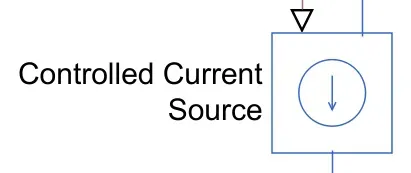
Current Sensor :-

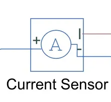
The current sensor block represents an ideal current sensor and is used to convert the current measured in an electrical circuit to a physical signal that is proportional to the current. This block is used to measure the current between the battery circuit (controlled current source) and the DC motor. The current sensor block is shown below:-

SOC & Current :-

• SOC stands for state of charge and it is a measurement of the available charge in a battery. 
•  When a battery is fully charged, it is considered to have a 100% charge and conversely 0% charge if fully discharged. In this EV model, I want to measure the current and the SOC of the battery as the simulation is run.
• I have used a scope block which shows the output signal we wish to measure as a plot against time. 
•  2 scopes have been used, one for the current and the other for the SOC. In order for this to be measured, we need to use a 'PS - Simulink converter' block. 
•  This is because the current signal is a physical one and we are measuring it as a logic signal in the SIMULINK workspace. 

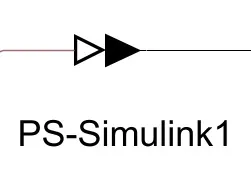
The PS-Simulink converter block is shown below:-

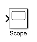
The scope block is shown below:-

SOC Subsystem :-

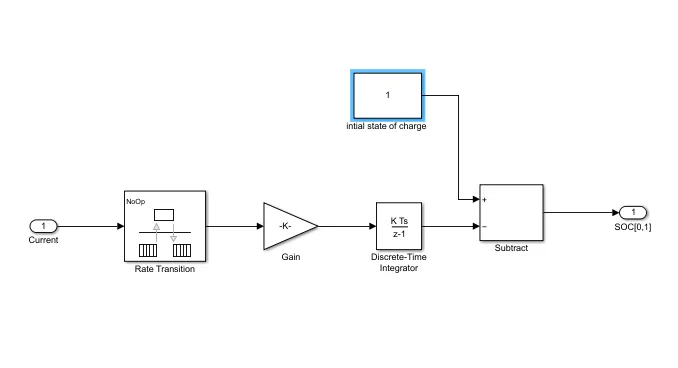
• To measure the state of charge of the battery, a subsystem was created of various blocks.
• The first block is the 'Rate Transition' block and it is used to handle data transfer between different rates and tasks.
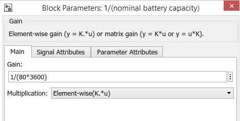
•  a 'Gain' block is used in order to multiply or divide the signal coming from the rate transition block. In this case, the gain block will divide the current signal with the ampere rating of the battery which has been taken as 80Ah multiplied by 3600 (seconds in an hour). 

• Then, a 'Discrete - Time Integrator' block is used to perform a discrete integration of the current signal with respect to the time. 
• A constant block is used to represent the initial SOC of the battery. Assuming that the battery is always fully charged when performing a simulation, I have altered the constant block with a value of 1 representing 100%. 
•  Next, a 'sum' block is used to perform addition and subtraction operations. The signal from the 'discrete time integrator' block will be subtracted from the constant block representing 100% charge. These components are connected as shown below.

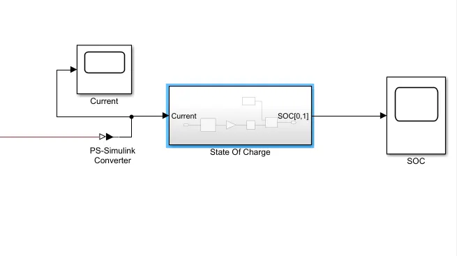
These blocks are then made in to a subsystem called 'Sate of Charge' and linked with the battery circuit using the PS-Simulink converter block. A scope block is used at the junction of the PS-Simulink converter block to plot the output signal of the current from the battery. Another scope is used to plot the output signal of the SOC from the SOC subsystem. This is shown in the image below:-

Speed Measurement :-

• In order to measure the speed of the EV model, I needed to use the scope block once again. I modified the scope block to have 2 input ports where one port takes the output velocity signal from the vehicle subsystem block and the other port takes the output signal from the drive cycle to the reference velocity port on the longitudinal driver block.
• This has been done so that the scope can show us the plots of the reference velocity and the actual velocity of the vehicle to see how they compare with each other. 

Distance Measurement :-

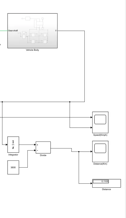
• I have used the scope block and mathematical operator blocks to measure the distance travelled by the vehicle according to the drive cycle data. 
• The area under a velocity time graph tells us the distance travelled by an object and so in my model. This means that the integral of the velocity with respect to time, gives us the distance travelled. 
•  So, I have implemented the integrator block to integrate the velocity signal that is output from the vehicle subsystem. 

The integrator block is shown below:-

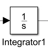
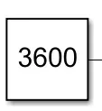
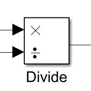
• From the integrator block, I needed to use the 'Divide' block along with a 'Constant' block having a value of 3600 in order to convert the divide the integrated speed signal which is in kilometres per hour by 3600.This will give us the distance travelled in kilometres. 

The 'Divide' block:-

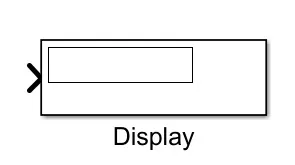
Finally, a 'Display' block is used to show the distance travelled as the simulation is run. The display block is shown below:-

If these blocks have been added to the workspace, they can be connected as shown in the image below:-

If all of these connections have been made, we can begin running the simulation for my EV model. 

Module :-

Results :-

I ran the WOT drive cycle for my EV model and took the outputs given from the speed, current and SOC scopes. The distance travelled by the vehicle in the drive cycle was also measured using the display block. Before running, the 'Stop Time' for the simulation was first set to 30 seconds which is the duration of my customized WOT drive cycle. 

Speed Scope :-

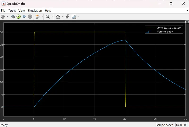
• From this scope, we can see 2 signals. The Yellow signal represents the reference signal which originates from the drive cycle data whereas the blue signal shows the actual velocity of the vehicle. The WOT drive cycle had been customized so that the vehicle begins.
• acceleration under the WOT condition (i.e.. full power) at t = 5 seconds. This is supposed to be maintained till t = 20 seconds when the vehicle is supposed to begin deceleration. From t = 20 seconds to t = 30 seconds, the vehicle speed is back to 0m/s i.e.. rest.
•  Because this is a reference signal, all the commands are instantaneous. This is why the increase and decrease in speed is very sudden within a fraction of a second. 
• However, this effect will not be observed on the actual velocity of the vehicle. This is because in real world conditions, there are more considerations to factor in which will not make it possible for a vehicle to accelerate and decelerate as instantaneously as the drive cycle commanded. In the real world, the effects of rolling resistance, drag and road inclination make a difference because their presence would cause the vehicle's motion to deviate from the drive cycle commands. Other factors include, the vehicle's inertia and the inertia of the transmission system. 
• Observing the vehicle's actual velocity, as commanded, the vehicle begins at rest before accelerating under the WOT condition at t = 5 seconds. This acceleration is maintained till t = 20 seconds as the drive cycle commanded.
• At t= 20 seconds,the vehicle achieves a top speed of 26.8m/s.  After t = 20 seconds, the vehicle begins to decelerate gradually till t = 30 seconds where the vehicle finishes with a velocity of approximately 7m/s.
• As mentioned earlier, the actual velocity could not match the drive cycle commands perfectly and this is due to several factors which were discussed above. In my model, I have not modelled a road inclination but I have used a wind velocity of 5m/s. I compared the effect of this wind resistance on the top speed of the vehicle to when there was no wind resistance. The effect was very insignificant, only affecting the top speed by 0.5m/s. 
•  Obviously, the model is limited to the simulation time allotted. So if a longer simulation time is used, the vehicle may reach a higher top speed and may even decelerate back to rest.

Current Scope :-

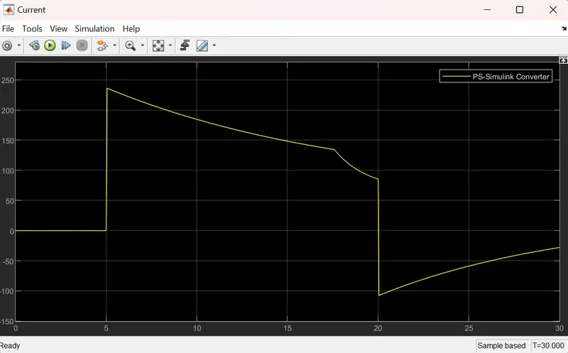
• The current scope shows how the current flowing from the battery to the motor varies with the drive cycle time. 
• initially the current flowing through the circuit is 0A and this corresponds to the drive cycle commanding the vehicle to be at rest for this time period. At t = 5 seconds, when the vehicle is commanded to accelerate, the current instantaneously increases to a maximum current of 236.1A.
• This maximum current is achieved because at t = 5 seconds, the vehicle accelerates at maximum power under the WOT condition and so this will demand a high current from the battery. From t = 5 seconds to t = 17.5 seconds, the current decreases gradually to 134.3A.
• The current must have decreased over time because as the vehicle was accelerating, it required lesser current from the battery to continue accelerating. The highest current is always required when accelerating from rest due to the inertia of the vehicle. 
• But once the vehicle is already in motion, it requires significantly lesser energy to continue accelerating. From t = 17.5 seconds to t = 20 seconds.
• The current flowing from the battery decreases more rapidly to 85.6A. This is because at this time, the acceleration of the vehicle began to level off meaning that the increase in speed in those 2.5 seconds was lesser than the increase from t = 5 seconds to t = 17.5 seconds. 
•  After t = 20 seconds, the vehicle decelerates, causing the current to drop instantaneously to the negative axis to a value of -107.4A. 
• There is now a negative current flowing due to regenerative braking. When the vehicle decelerates, the throttle is no longer applied and so the kinetic energy from the motion is converted to electrical energy fed back to the battery of the EV. This reverse flow of current is what causes the negative current measurement.
• From t = 20 seconds, the deceleration continues, however the current flowing through the battery decreases in magnitude. This is because at t = 20 seconds, the vehicle had reached its top speed and hence its maximum kinetic energy. 
•  So, at that point there was more kinetic energy which could be converted to electrical energy for regenerative braking. However, as the vehicle decelerates, there was lesser energy available for regenerative braking causing the magnitude of the current to decrease. The polarity of the current hence moves towards the positive direction because regenerative braking happens lesser and lesser until the vehicle comes to rest. At t = 30 seconds, the vehicle is still decelerating and finished with current measurement of -27.9A showing that regenerative braking is still occurring.

SOC Scope :-

 

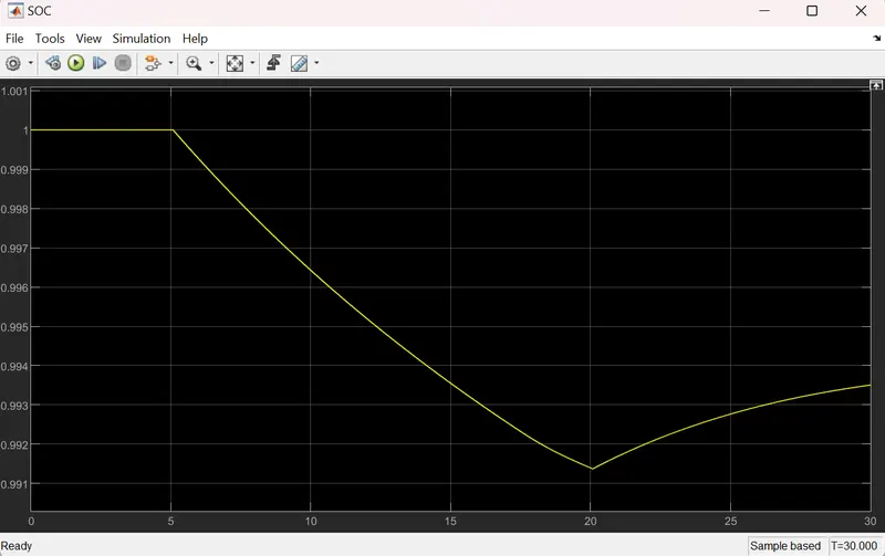
• The SOC scope shows how the state of charge of the battery varies over the drive cycle time. The battery was modelled to begin with an SOC of 1 (100%) and so when the simulation begins, the SOC is at 1 until t = 5 seconds. 
• At t = 5 seconds, the vehicle is commanded to accelerate under the WOT condition and so the SOC of the battery decreases. Because the vehicle is accelerating at full power, the SOC falls from 1 but the rate of discharge decreases over the acceleration period eventually settling at a minimum SOC of 0.9914 at t = 20 seconds.
•  This corresponds to the current flow from the battery because as the vehicle accelerates, lesser energy is demanded to increase the speed.
• At t= 20 seconds, the vehicle is commanded to decelerate and so the vehicle velocity decreases. This results in regenerative braking to occur which causes a negative flow of current back to the battery.
• Because this effect charges the battery, the SOC of the battery increases during the deceleration period. The SOC increases very gently from 0.9914 to 0.9935 and this is because the gets charges by the regenerative braking effect. 
• The negative flow of current corresponds to the increase in the SOC of the battery. Since the vehicle is commanded to decelerate until t = 30 seconds, the vehicle speed decreases but does not reach 0m/s, so the vehicle is under regenerative braking for the entire period after t = 20 seconds.

Distance Measurement :-

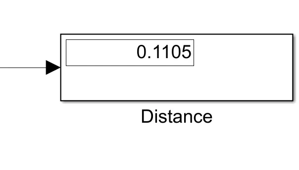
• From the image above, we can see that the display block has measured the distance travelled by my EV model for the customized WOT cycle to be 0.1105km.
• This measurement seems appropriate and correct since the WOT drive cycle is very short in duration and only requires acceleration for half of the drive cycle's overall duration. The area under the velocity time graph tells us the displacement of an object. From looking at the speed scope, a rough calculation indicates that this distance measurement is correct.
• Displacement is defined as distance in a given direction and is a vector quantity meaning it has both size and direction. So, if the velocity data in a drive cycle was negative, this would indicate that the vehicle is moving in the reverse direction and this would correspond to a negative displacement. The display block would indicate the same if the velocities in the drive cycle data were of that nature. 

Conclusion :-

• the EV model has been created with the necessary block components using the SIMULINK software and the model has been simulated for a customized WOT drive cycle.
• The simulation has produced results of the velocity of the vehicle, current flowing from the battery, and the SOC of the battery as well as the distance travelled by the EV. Since the EV model was parameterized to simulate averaged voltage pulses in the H-Bridge and Controlled PWM voltage blocks to be fed in to the DC motor, the simulation was run very quickly within a matter of seconds. 
• The EV model was able to follow the commands given by the reference velocities from the drive cycle data, although it could have followed the reference signals more closely. The discrepancy between the reference velocity and actual velocity of the vehicle may be attributed to a variety of factors e.g. vehicle inertia, transmission system, transmission inertia.
• If the EV model was designed in such a way as to improve upon those factors, the model would follow the reference signals more closely and would improve the performance characteristics as well. The distance travelled by my EV model was measured at 0.1105km and seems to be an appropriate value based on the (Wide Open Throttle) drive cycle used.
• I had observed that the SOC of the battery used in my EV model did not get discharged in a way I had expected it to. This could be because the drive cycle commands did not push the EV model to its limits or it could be due to the fact that the battery model was very efficient and was suitable for the driving application.
• My EV model had also included some actual features of EVs such as regenerative braking and this was evident in the current - time and SOC - time graphs whenever the EV decelerated. If the duration of the WOT drive cycle was modified to be longer, I could have seen my EV model exhibit its true performance characteristics. For instance, the EV model may achieve its top speed and it may also have been possible to see the time it takes for the vehicle to decelerate from that top speed and hence the time taken for the acceleration e.g. 0 to 60 kmph. 

Reference :-

Youtube video,

https://youtu.be/tM9Akdo8QeA

https://youtu.be/xmdUFEfiAKk