Project - Speed Control of a Direct Current (DC) motor
PROJECT:- In this project, a Simulink model for the DC motor will be first developed per the schematic shown in Figure 1.
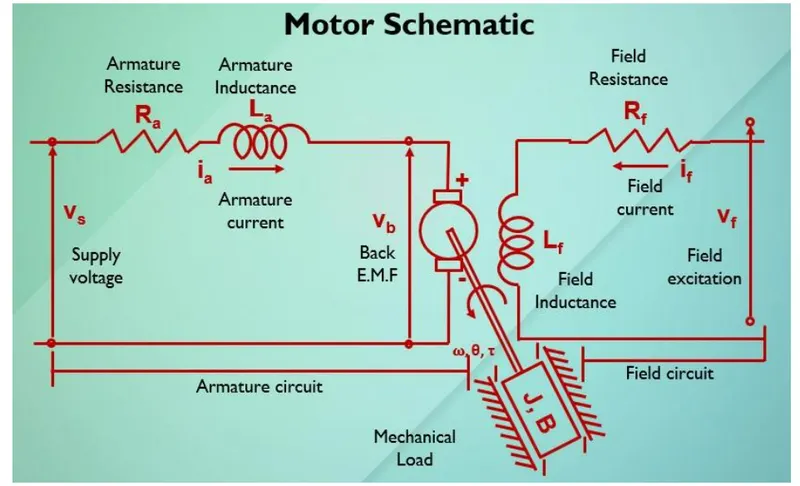
For this above schematic Diagram ,we will assume the Input odf the dc moter is Voltage source(Vs) and out of the moter is Rotational speed (w) of the moter shaft.
>>Both the rotor and shaft are to rigid then we gets the Viscus friction(J) and Torque(T).
>> The Torque (T) of the motor is prapotional to the armature Current (ia) with torque Constant (Kt)
i.e., T=Kt * ia-----------(1)
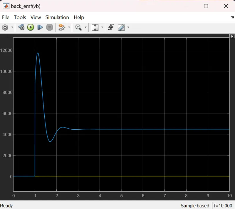
>> Back EMF (Vb) is praportional to angular velocity (theta_dot) by a praportional constatnt (Kb)
i,e., Vb = Kb * (theta_dot)----------(2)
>>For creating the The SIMULINK MODEL of above given DC moter let us find the transfer funcion as followes ::-
From the schematic diagram we have apply kirchoff's Voltage law To the Armature Circuit.
Armature Circuit Equatation Part :-
Vs= Ra* ia + L (dia/ dt) +Vb ----------(3)
substitute eqn (2) in eqn (3) then we get
Vs= Ra* ia + L (dia/ dt) +(Kb* (theta_dot)-----------(4)
Vs-(Kb* (theta_dot)=Ra* ia + L (dia/ dt)------------(5)
From Equatation (5) we can write as :-
L( d ia / dt ) = (Vs-(Kb* (theta_dot)-Ra*ia)-----------(6)
Field Circuit Equatation Part:-
Appling the Newton's Law of Moton for Field circuit Then we get:-
J(d^2 theta /d t^2) + B (d theta /d t)= Kt * ia---------------(7)
Aplly Laplace Transforms to both equatations (6) and (7) then :-
from eqn (6) :-
L I(S)=V(S)- Kb (theta (S)- Ra I(S)
L I(S)+ Ra I(S)=V(S)- Kb (theta (S)
I(S) (L+Ra)=V(S)- Kb (theta (S)
I(S)=V(S)- Kb (theta (S) / (L+Ra)-----------------(8)
From eqn (7):-
J S^2 (theta (S))+ B s (theta (S)) =kt * I(S)---------------(9)
substitute I(S) value in eqn (9) then we get :-
J S^2 (theta (S))+ B s (theta (S)) =kt *{V(S)- Kb (theta (S) / (L+Ra)}
S * theta (S) ( J S +B)=kt *{V(S)- Kb (theta (S) / (L S+Ra)}---------------------(10)
From equatation (10) We get transfer function between output (w(s)) Angular velocity and input volatge (Vs) as followes :-
W(S) / Vs = Kt / {(L S+Ra) (J S + B)+Kt* Kb}-----------------(11)
Mathematical modeling from the first principles:-
From eqn (11) this we can design the SIMULINK MODEL:-
W(S) / Vs = Kt / {(L S+Ra) (J S + B)+Kt* Kb}
From This transfer function we can design the DC_MOTOR Mathematical model as followes :-
SIMULINK BLOCKS :-
Clock:-To return the time as output signal
To work space:-To save the output in workspace
gain :-To return the output signal as gain of input signal
sum:- to return the output signal as sum of input signal
step:-to generate pulse signal(source voltage vs).
Transfer funcrion :-To return the out as transfer function format of input given signals.
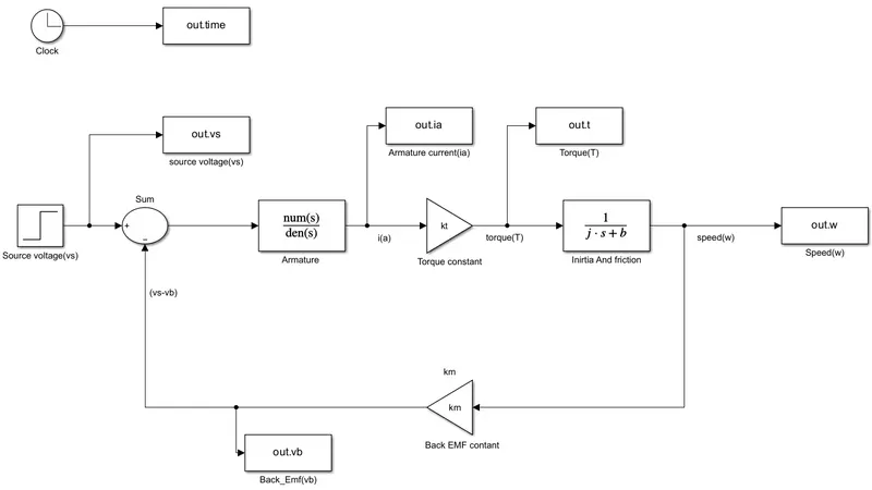
fig(1)
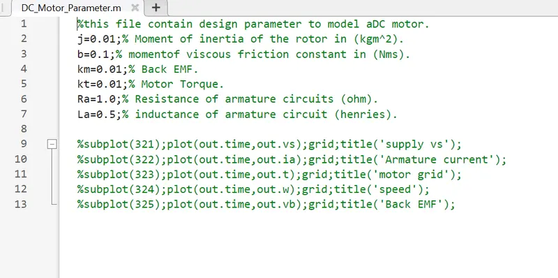
PRAMETERE(Design):-
OUTPUT (Graph):-
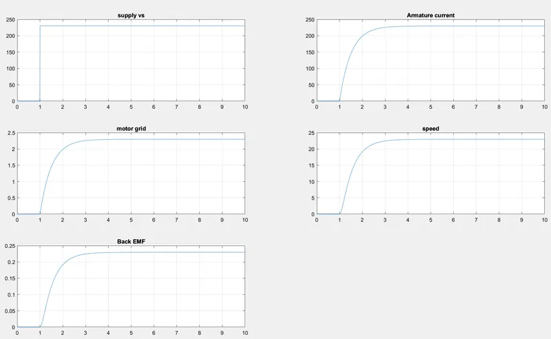
- THIS ENTIRE BLOCK CAN BE CONVERTED INTO (SINGLE-SUBSYSTEM) USING FOLLOWING STEP:-
Step 1:- select all block of above model (DC-model).
Step 2:- After selecting all block, right click ''Create subsystem from selection'' then we got all block in
signal subsystem model.
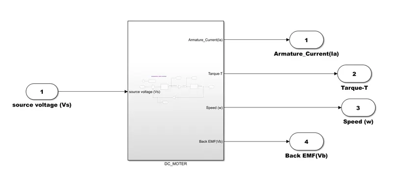
fig(2)
Use the Proportional, Integral, and Derivative (PID) control design knowledge gained in the training
to design, develop and test a controller to maintain a desired speed for the motor.
SIMULINK BLOCKS :-
Clock:-To return the time as output signal
To work space:-To save the output in workspace
gain :-To return the output signal as gain of input signal
sum:- To return the output signal as sum of input signal
step:-To generate pulse signal(source voltage vs).
Integrator:-To return the output signal in form of integration of input signal.
Scope:- To represent the output in form of Graph.
PID_CONTROLLER_BLOCK:-
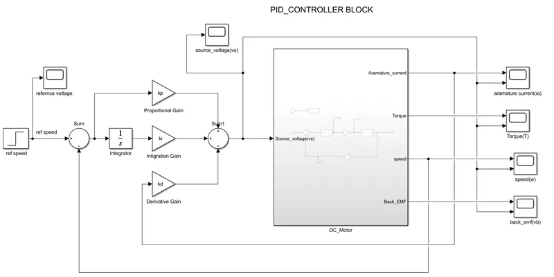
fig(3)
PARAMETERS(are assumed for example) :-
MATLAB SCRIPT(above given value).
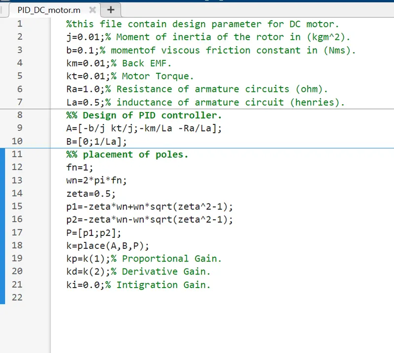
OUTPUT:-
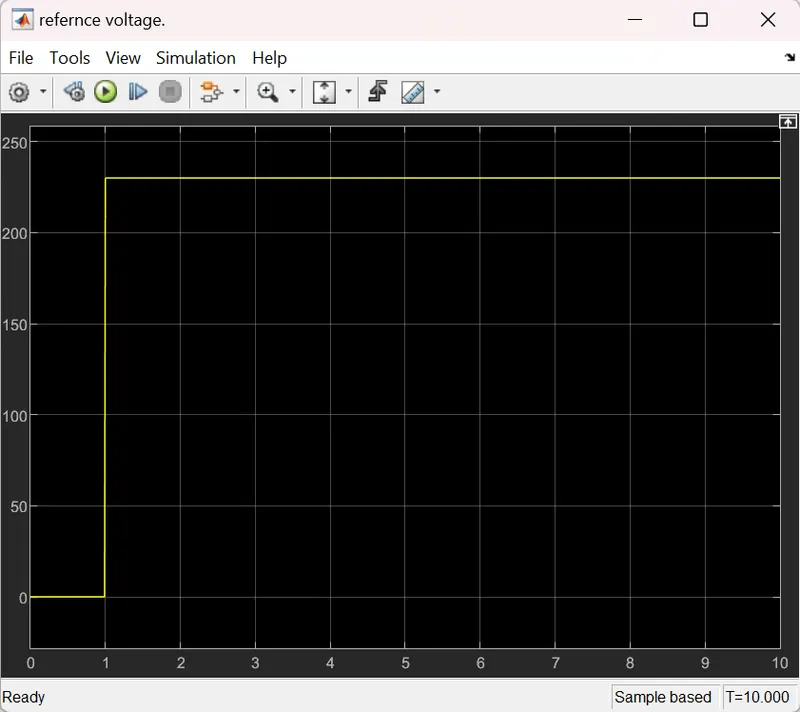
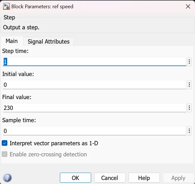
REFERCENCE VALUE IS START THE STEP OF 1 AND UPTO 230 THEN IT GET EQUILBRIUM POSITION.
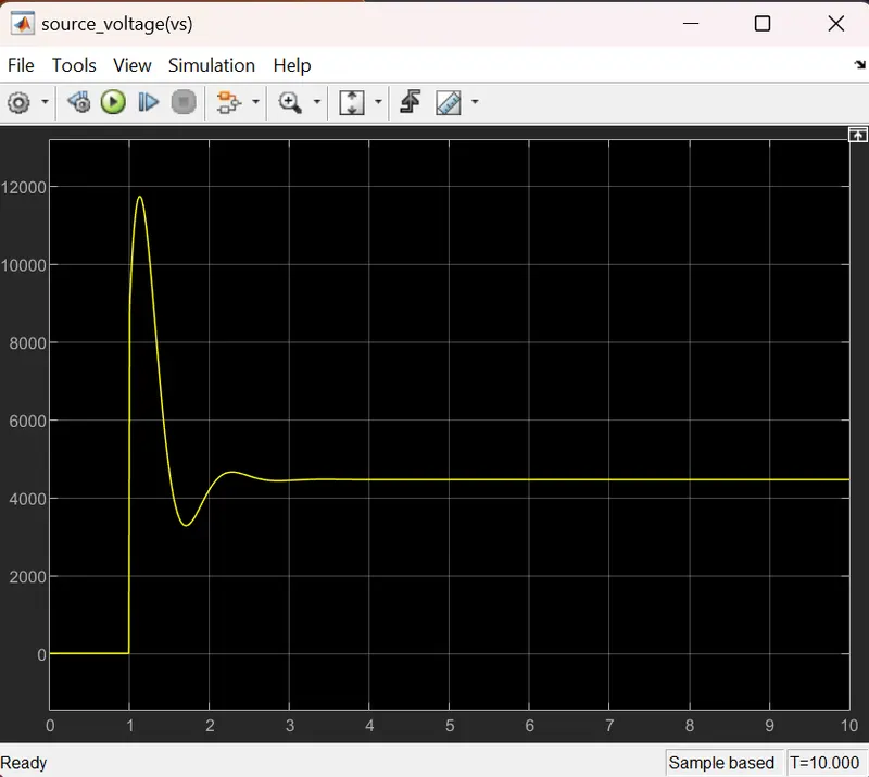
SOURCE_VOLTAGE(VS)_SCOPE:-
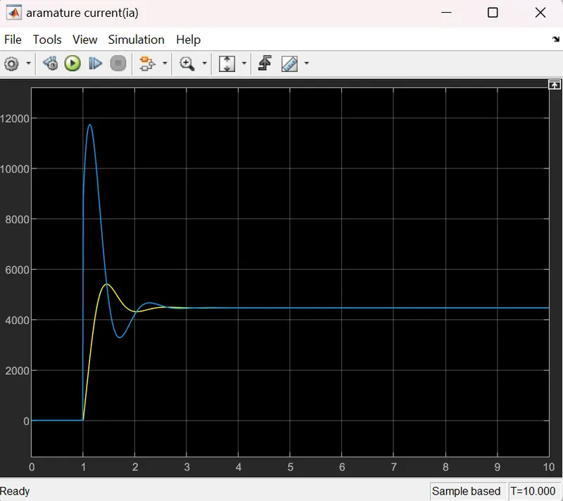
ARMATURE_CURRENT(IA):-
BACK_EMF(Vb):-
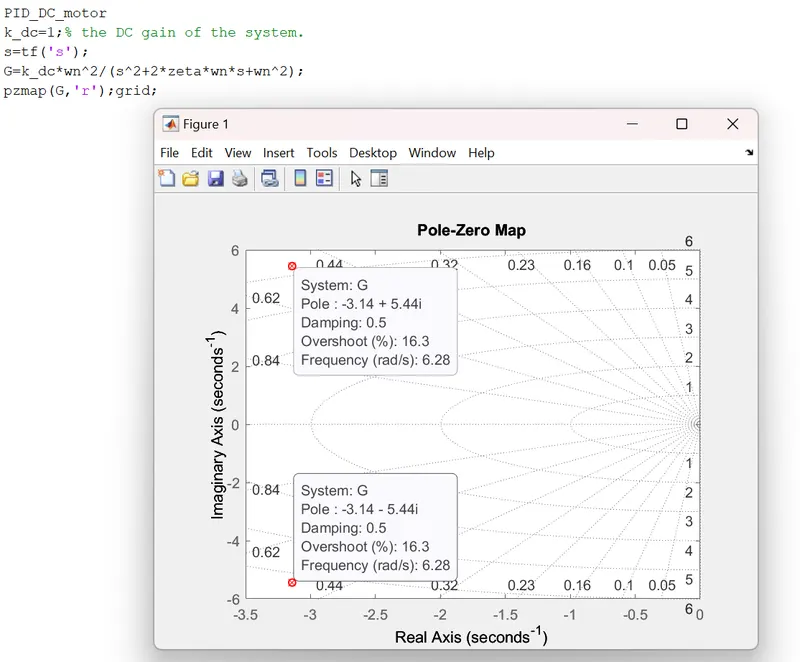
GIVEN TRANFER FUNCTION THE POLES:-