Design of an Electric Vehicle
Aim
To create a MATLAB model of electric car which uses a battery and a DC motor
Objectives
- To make a most simple and low run time vehicle model using individual components
- To check out performance parameters
- To check the model results
- To know MATLAB models and concluding their configurations
Introduction
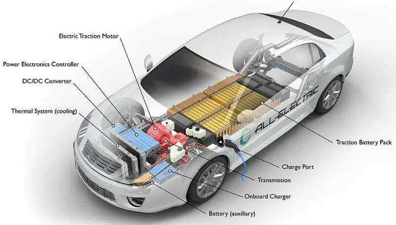
Electric cars run on electricity. Unlike conventional vehicles that use a gasoline or diesel-powered engine, electric cars use an electric motor powered by electricity from batteries or a fuel cell. Electric cars store electricity onboard with high-capacity battery packs. Their battery power is used to run the electric motor and all onboard electronics.
Simple representation of the vehicle can be done by a block diagram and it is given below.
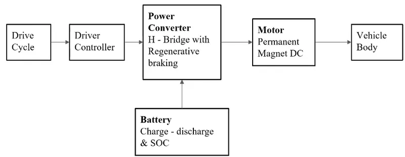
From the above diagram we will get a overall idea of the model of the vehicle. Now we can model the vehicle
Modelling and Simulation
→ System configuration
Model of the electric vehicle which was created is represented below.
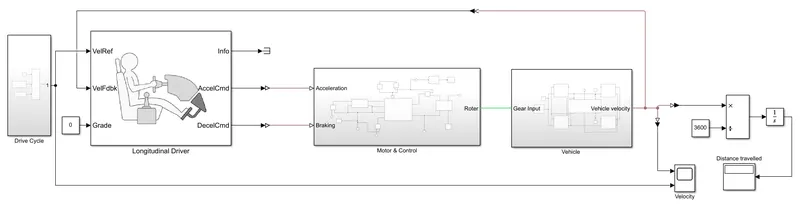
Firstly, the vehicle body was created and it was changed into a subsystem. Similarly, DC motor and related configurations were also created as a subsystem. Proper blocks were used to connect these and final model represented above was obtained.
→ Model parameters
Drive Cycle: Every vehicle needs a drive cycle so that we can simulate the performance. It will act as a drive input for the iterations. The drive cycle system which was created is given below.
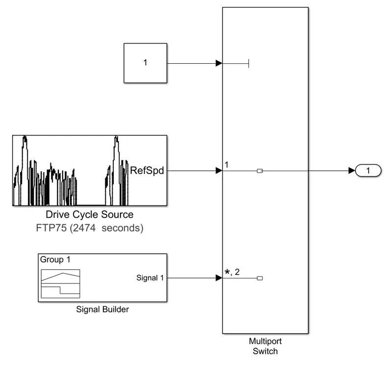
It consists of a drive cycle source and a signal builder. These two blocks are connected to a multiport switch so that we can select one of them. Drive cycle source block generates a standard longitudinal drive cycle. The block output is the vehicle longitudinal speed. Here we have selected FTP75 cycle and it is given below.
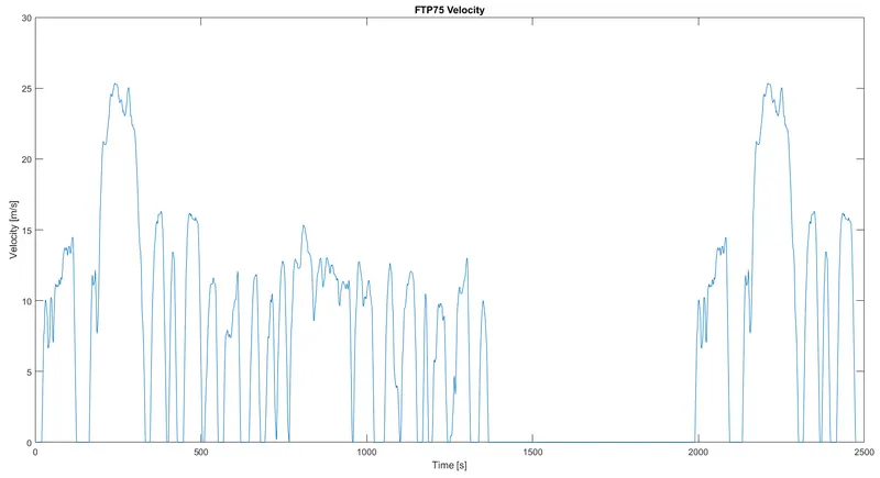
We can also give a customized drive input with the help of signal builder block. The selected drive input is given to the longitudinal driver block as a reference velocity.
Longitudinal Driver: It is a parametric longitudinal speed tracking controller for generating normalized acceleration and braking commands based on reference and feedback velocities. We have already given the reference velocity as drive cycle. In this block, we can add any grade values if we want. Acceleration and braking outputs are connected motor controlling unit.
Motor & Controller: This subsystem drives the shaft according to the input of driver. The representation of the subsystem is given below.
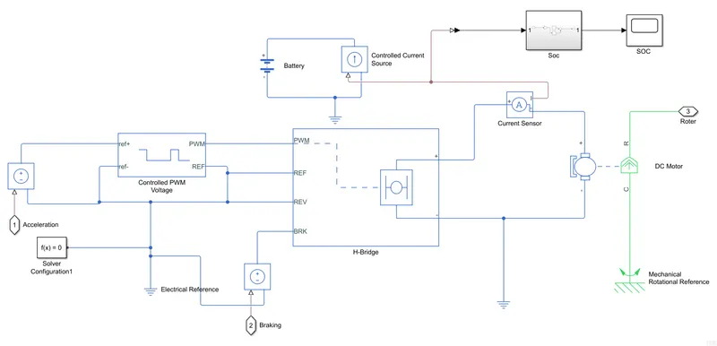
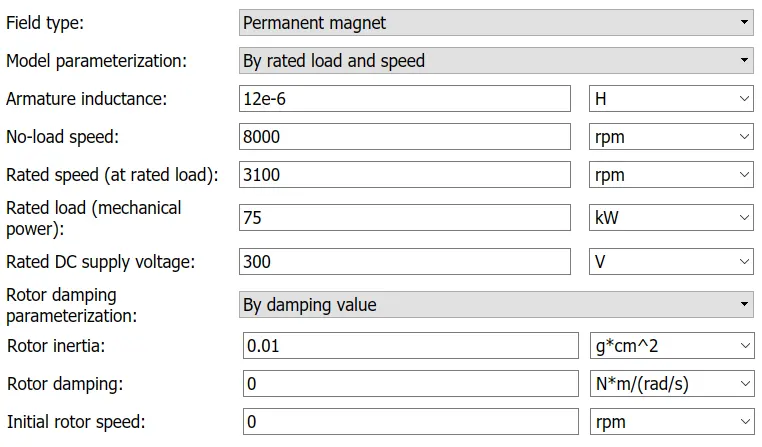
Here we used a DC motor to power the model. The parameters for the motor is given below.
DC motor is controlled by an H bridge block. The block can be driven by the Controlled Pulse Width Modulator (PWM) Voltage block. We selected the average mode for PWM block. In Averaged mode, the PWM port voltage divided by the PWM signal amplitude parameter defines the ratio of the on-time to the PWM period. Using this ratio and assumptions about the load, the block applies an average voltage to the load that achieves the correct average load current. We kept the Simulation mode parameter value for the Controlled PWM Voltage and H-Bridge blocks same. If the REV port voltage is greater than the Reverse threshold voltage, then the output voltage polarity is reversed. If the BRK port voltage is greater than the Braking threshold voltage, then the output terminals are short circuited via one bridge arm in series with the parallel combination of a second bridge arm and a freewheeling diode. Voltages at ports PWM, REV and BRK are defined relative to the REF port. The parameters for the H bridge is given below.
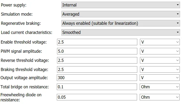
The PWM block will keep the output voltage zero when the pulse is low, and equal to the output voltage amplitude parameter when high. Duty cycle is set by the input value. A controlled current source is given to the modulator so that the power will not be used uncontrollably. Battery is also connected to the DC motor with a monitoring system for the battery. It is a subsystem named SOC.
SOC: State Of Charge (SOC) is the level of charge of an electric battery relative to its capacity. This block is used to find out the level of battery after the vehicle completes the drive cycle. The system representation is given below.
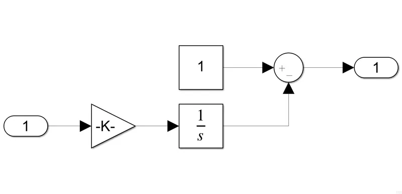
We can get the state of charge of the battery from the scope block connected to it. The rotor output of the motor is given as a input to the gear system in the vehicle subsystem.
Vehicle: This subsystem resembles the body of electric car and its representation is given below.
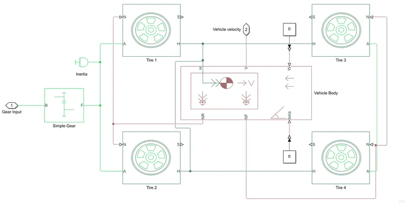
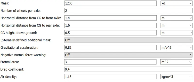
The vehicle body block represents a two-axle vehicle body in longitudinal motion. The block accounts for body mass, aerodynamic drag, road incline, and weight distribution between axles due to acceleration and road profile. Connection H is the mechanical translational conserving port associated with the horizontal motion of the vehicle body. The resulting traction motion developed by tires is connected to this port. Connections V, NF, and NR are physical signal output ports for vehicle velocity and front and rear normal wheel forces, respectively. The vehicle body parameters are represented below.
Connections W and beta are physical signal input ports corresponding to wind speed and road inclination angle, respectively. Gear input is given to the wheel blocks. We will get the vehicle velocity from the output port and it is given to the longitudinal driver block as feedback velocity. The feedback and reference velocities are connected to a scope block so that we can compare them. Output velocity is also integrated and converted to distance in kilometres by an integrator block.
Results
The results obtained from the simulation are given below. First one is the velocity plot. Blue line indicates the velocity of the vehicle and red one denotes the drive cycle.
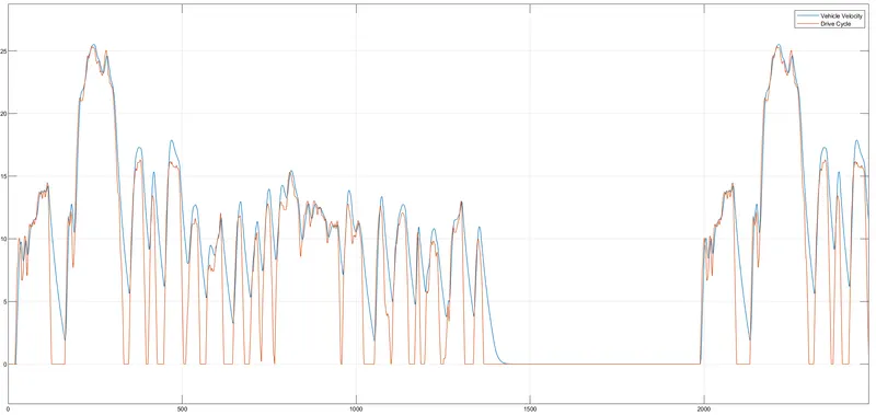
From the plot it is clear that, the vehicle is almost following the drive cycle. But if we observe closely, in some regions vehicle demands little more speed than the drive cycle and in some regions it is not becoming zero as per the drive cycle. Vehicle came to rest with drive cycle only when there was sufficient time. Maximum speed of the drive cycle is 25.35m/s. From the plot, vehicle demands little more than that. If we look the deceleration part, vehicle takes more time to reduce its speed because of its inertia. Now we can look in to the distance travelled by the vehicle. It is obtained from the display which was conected. The representation is given below.
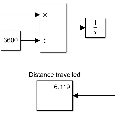
The vehicle travelled 6.12km. Average speed of the drive cycle was 9.5m/s. So with this speed, vehicle travelled for six kilometers and our battery alomost drained out. The soc plot is given below.
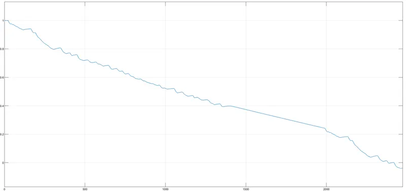
In some small regions, we can see the plot is holding steady. This is beacause of regenerative braking.
Conclusion
We were able to model a simple and low run time vehicle model using individual components. This simple model is capable of running 6km with full charge. Even if this model is not a practical model, it is very effective for getting simulation data in very less time. If we change the configuration of the model, we can surely make this model similar to practical case models.
Reference
[1] https://afdc.energy.gov/vehicles/how-do-all-electric-cars-work